Introduction to Unstructured Data

⚡️ Our code from class is now available here

What is Unstructured Data?

When working with data, you’ll often come across the terms “structured” and “unstructured” data. There are lots of definitions online, like this graph below:

structured vs unstructured

This graph is technically correct, but it is also a bit confusing when you think about it (even highly organized data can be difficult to analyze for example and why can’t things like email be analyzed in spreadsheets?).

Let’s compare our two datasets that we have been working with so far: the Film Dialogue dataset and the Humanist Listserv dataset.

In our Film Dialogue datasets, we have technically four separate spreadsheets with the following columns:

Public Script Sources - public_scripts.csv with:

`imdb_id`	`script_id`	`title`	`year`	`gross_ia`	`link`
tt0019777	4031	The Cocoanuts	1929	nan	http://www.pages.drexel.edu/~ina22/splaylib/Screenplay-Cocoanuts,_The.pdf

character_list5.csv with :

`script_id`	`imdb_character_name`	`words`	`gender`	`age`
280	betty	311	f	35

character_mapping.csv with:

`script_id`	`imdb_id`	`character_from_script`	`closest_character_name_from_imdb_match`	`closest_imdb_character_id`
1	tt0147800	bianca	bianca stratford	nm0646351

meta_data7.csv with:

`script_id`	`imdb_id`	`title`	`year`	`gross`	`lines_data`
1534	tt1022603	(500) Days of Summer	2009	37	743544525677477444334257777565774443444456445674543367553452777734237544553444343334444444467441433777777777777776634344344434244343433435535624644435776576434333377775756764434344466346764533566544444777533356445543543343334444535476332345777777777777776

In our Intro to EDA notebook, we discussed how some of the values in these spreadsheets are categorical values (like gender as a nominal category – that is discrete unordered categories) and how some are numerical values (like gross or lines_data). And finally how some are a bit in between, like year which is technically represented as a number and we could treat it as either a continuous or discrete value, or we could treat it as a categorical value that is ordinal (i.e. is a category with an implied order).

The big thing to takeaway from looking at these datasets though is that all these values are structured. We do not need to do any processes to turn these values into data to analyze. We might group them, we might filter them, we might fill in missing values, and we can plot them – but essentially this is a dataset ready to be analyzed.

Let’s compare that to our Humanist listserv dataset.

With web_scraped_humanist_listserv.csv we have:

`dates`	`text`	`url`
1987-1988	From: MCCARTY@UTOREPAS\nSubject: \nDate: 12 Ma…	https://humanist.kdl.kcl.ac.uk/Archives/Converted_Text/humanist.1987-1988.txt

I’ve truncated the text file column for visual clarity, but overall this is a much less complex dataset than the Film Dialogue dataset. We could leave the dataset as is and treat it as structured or semi-structured data but our analysis would likely be very limited since we have no numeric data.

Instead to make our Humanist Listserv dataset into something like the Film Dialogue datasets, we need to go through a process of curating and cleaning the data from unstructured to structured data, similar to this graph below:

data humanities knowledge continum

It’s worth noting here that this structured vs unstructured divide is very porous and ill defined, and mostly has a lot to do with your goals and your data.

Structuring our Textual Data

So let’s try adding some structure to our Humanist Listserv dataset. Let’s start a new notebook called HumanistListservEDA.ipynb and import our libraries and data.

Now we need to start thinking about the types of data that we have and exploratory data analysis we might want to undertake.

First we can check our data types:

# Check the data types of our columns
humanist_vols.dtypes

We should see the following output:

dates    object
text     object
url      object
dtype: object

In Intro to Notebooks, we learned that Pandas treats string data as object data (also all mixed numeric or non-numeric values). So now we know that to work with our data we will need to dig into Pandas string methods. An in-depth discussion of these methods are available on the Pandas documentation website https://pandas.pydata.org/docs/user_guide/text.html, but I’ve also summarized many of the more popular methods below in this table:

Pandas String Method	Explanation
`df[‘column_name’].str.lower()`	lowercase all the values in a column
`df[‘column_name’].str.upper()`	uppercase all the values in a column
`df[‘column_name’].str.replace(‘old_string’, ‘new_string’)`	replace all instances of ‘old_string’ with ‘new_string’ in a column
`df[‘column_name’].str.split(‘delimiter’)`	split a column by ‘delimiter’ like a comma or period, or really anything
`df[‘column_name’].str.strip()`	remove leading and trailing whitespace from a column
`df[‘column_name’].str.len()`	count the number of characters in a column
`df[‘column_name’].str.contains(‘pattern’)`	check if a column contains a particular pattern
`df[‘column_name’].str.startswith(‘pattern’)`	check if a column starts with a particular pattern
`df[‘column_name’].str.endswith(‘pattern’)`	check if a column ends with a particular pattern
`df[‘column_name’].str.find(‘pattern’)`	find the first occurrence of a particular pattern in a column
`df[‘column_name’].str.findall(‘pattern’)`	find all occurrences of a particular pattern in a column
`df[‘column_name’].str.count(‘pattern’)`	count the number of occurrences of a particular pattern in a column
`df[‘column_name’].str.extract(‘pattern’)`	extract the first occurrence of a particular pattern in a column
`df[‘column_name’].str.extractall(‘pattern’)`	extract all occurrences of a particular pattern in a column
`df[‘column_name’].str.join(list)`	join a list of strings with a delimiter

This list is not exhaustive, but it’s a good starting point and shows that there are a number of approaches we could take.

Let’s start off with trying to explore the size of each volume over time. First, we need to split our dates column into a year_start and year_end columns.

# Split the dates column into year_start and year_end 
humanist_vols['year_start'] = humanist_vols['dates'].str.split('-').str[0]
humanist_vols['year_end'] = humanist_vols['dates'].str.split('-').str[1]

Now that we have our years, we need to get the size of each volume. We can do this by using the count method and thinking of a pattern that would represent size of the volume (maybe the frequency of new lines \n or FROM ?).

# Count the number of characters in each volume
humanist_vols['volume_size'] = humanist_vols['text'].str.count('\n')

Final step is to plot our data to explore the pattern we are interested in!

# Plot the data
humanist_vols.plot(x='year_start', y='volume_size', kind='bar')

We should produce a graph that looks like this:

humanist size

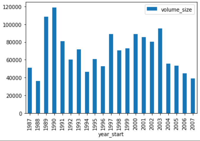
Wonderful! We both structured our data and completed our exploratory analysis. But one remaining issue is how could we start to ask questions about the content of our text data from the listserv? What patterns and themes are there in the text? That’s where text analysis comes in!

What is Text Analysis?

One of the main ways we can structure our Humanist listserv data is by undertaking something called text analysis. This is a very broad term for a whole set of practices and overlapping disciplines and fields, some of which are shown in this figure below:

text analysis

But again this figure has its limits. For example, data mining is something that Library & Information Sciences undertakes, and databases are used across these domains.

Rather than trying to define text analysis as a whole, I find a more helpful distinction is talking about Information Extraction vs Information Retrieval.

Information Retrieval (IR):

information retrieval

Goal of finding relevant documents for user’s needs/queries (eg. Google)
Often used for text classification of documents
Can be done without “understanding” syntax and treating documents as “bag of words”

Information Extraction (IE)

information extraction

Goal of extracting specific features from documents
Focused on linguistic analysis of textual features
Requires both syntactic and semantic analysis

Today we will be focusing on the first category of these two categories, Information Retrieval, and next week we will dig into Information Extraction.

What is Information Retrieval?

According toWikipedia, Information Retrieval (or IR) was first theorized in the 1940s:

origins IR

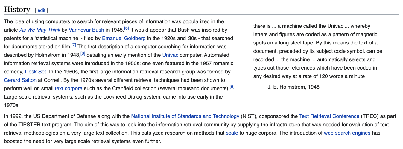
Information retrieval is strongly tied to the historical development of search engines and the basic goal is to find relevant documents for a user’s query. To do that though requires parsing textual information and finding patterns in the text.

One way we can do that is with simple counting of words and the frequency they appear across a text.

In our example, we could start counting words that appear in our email logs. Thinking back to some of our readings, we could try and compare the rate that humanities computing appears compared to digital humanities that we first explored in the Google Ngram Viewer, demonstrated below.

hc dh

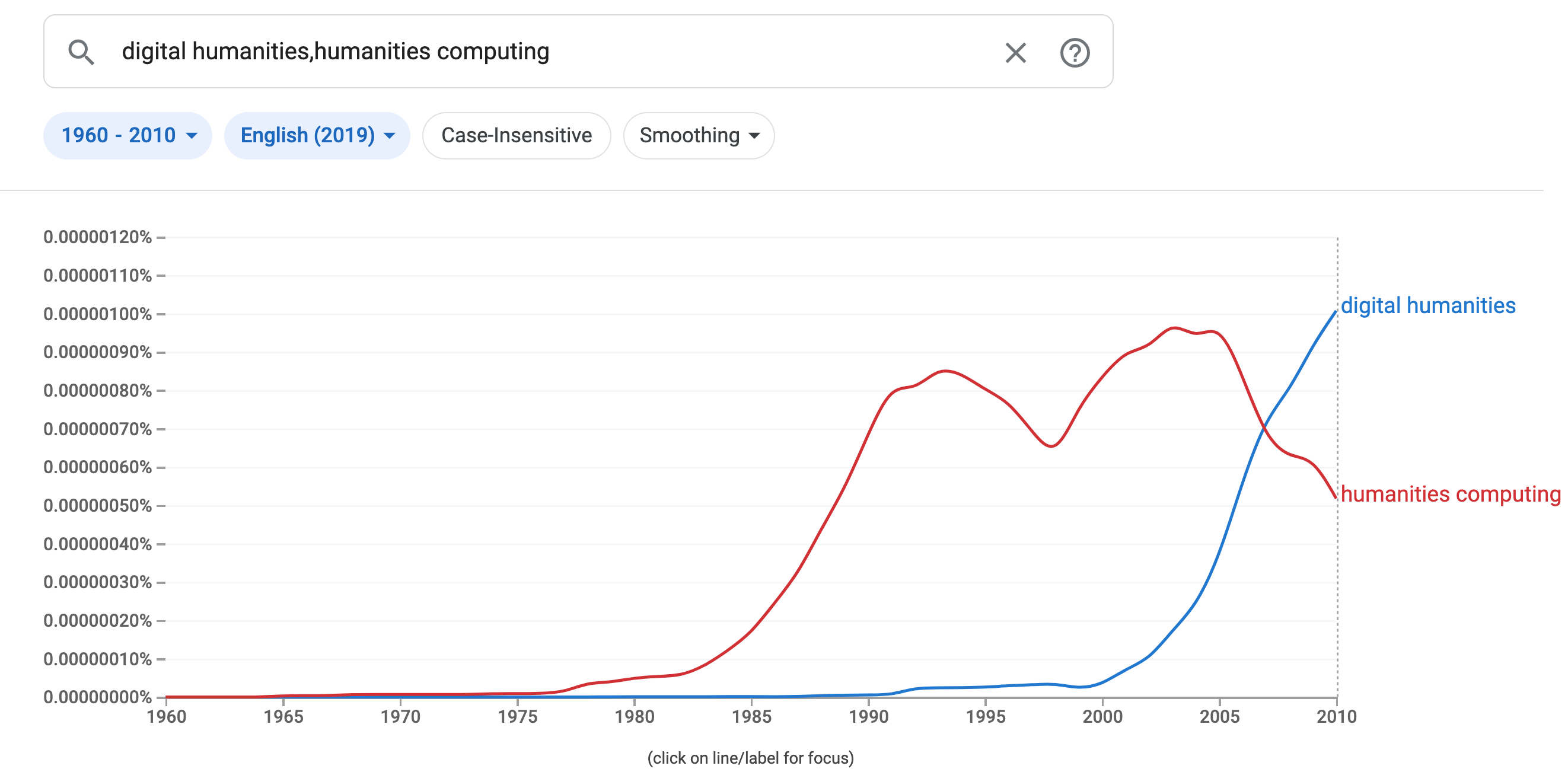
We can do a similar experiment in this listserv dataset. First we need to figure out how we can count strings in Pandas. We can do this by using the count method.

# Count the number of occurrences of each word
humanist_vols['humanities_computing_counts'] = humanist_vols['text'].str.count('humanities computing')
humanist_vols['digital_humanities_counts'] = humanist_vols['text'].str.count('digital humanities')

Now we can plot the data.

# Plot the data
humanist_vols[['humanities_computing_counts', 'digital_humanities_counts']].plot()

Which produces the following graph:

hc dh counts

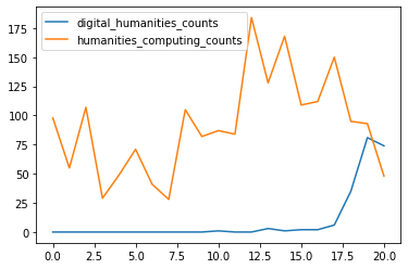
We’ve officially done our first foray into text analysis 🥳!

Text Analysis with Python

So far we’ve just been working with Pandas, but in Python, there exists a few libraries specifically designed to work with text data.

NLTK https://www.nltk.org/
SPACY https://spacy.io/
SCIKIT-LEARN https://scikit-learn.org/stable/

Each of these libraries has its own history, and some of what they provide overlaps. Here’s a helpful chart outlining some of their pros and cons.

comparison

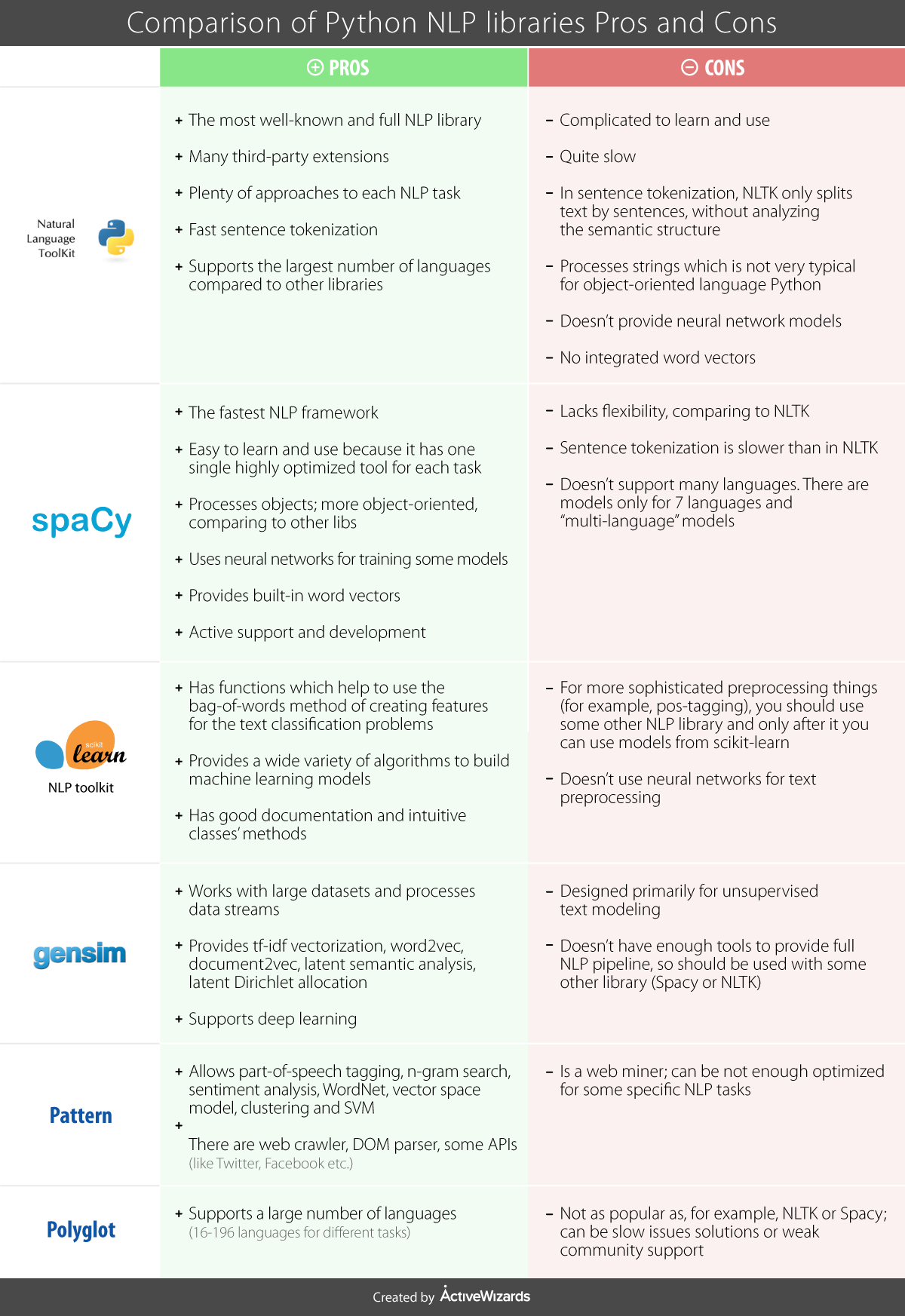
Ultimately, which library you choose to use depends on what you want to do with your data, but there’s some general principles for text analysis that you should consider regardless of method.

Word Counts and Zipf’s Law

The library NLTK has a helpful built in Class called FreqDist that takes a list of words and outputs their frequency in a corpus http://www.nltk.org/api/nltk.html?highlight=freqdist

Let’s try it out with a subset of our data. (Remember to install nltk).

from nltk import word_tokenize
from nltk import FreqDist

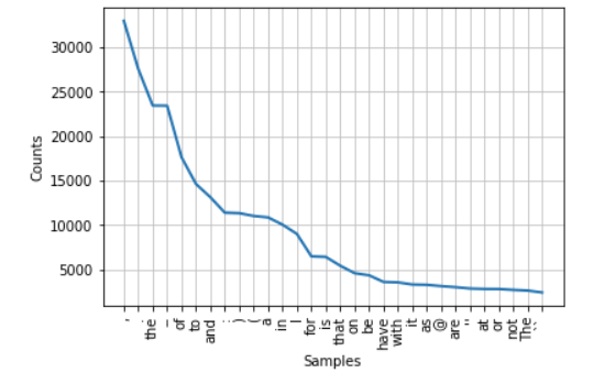
tokens = FreqDist(sum(humanist_vols[0:2]['text'].map(word_tokenize), []))
tokens.plot(30)

We should get a graph that looks like this: counts .

In this graph, if we had used all the words we would see this trend continue, like in the graph below.

zipf

This is “Zipf’s law:” the phenomenon means that the most common word is twice as common as the second most common word, three times as common as the third most common word, four times as common as the fourth most common word, and so forth.

It is named after the linguist George Zipf, who first found the phenomenon while laboriously counting occurrences of individual words in Joyce’s Ulysses in 1935.

This is a core textual phenomenon, and one you must constantly keep in mind: common words are very common indeed, and logarithmic scales are more often appropriate for plotting than linear ones. This pattern results from many dynamic systems where the “rich get richer,” which characterizes all sorts of systems in the humanities. You can read more about the power of counting words here https://tedunderwood.com/2013/02/20/wordcounts-are-amazing/.

Tokenization

In the field of corpus linguistics, the term “word” is generally dispensed with as too abstract in favor of the idea of a “token” or “type.” Breaking a piece of text into words is thus called “tokenization.”

There are, in fact, at least 7 different choices you can make in a typical tokenization process.

Should words be lowercased?
Should punctuation be removed?
Should numbers be replaced by some placeholder?
Should words be stemmed (also called lemmatization).
Should bigrams or other multi-word phrase be used instead of or in addition to single word phrases?
Should stopwords (the most common words) be removed?
Should rare words be removed?

Any of these can be combined: there at least a hundred common ways to tokenize even the simplest dataset.

We can try these out with our humanist_vols dataset. For example, would we get a different number of counts if we lowercased our words?

# Count the number of occurrences of each word lowercased
humanist_vols['lowercase_humanities_computing_counts'] = humanist_vols['text'].str.lower().str.count('humanities computing')
humanist_vols['lowercase_digital_humanities_counts'] = humanist_vols['text'].str.lower().str.count('digital humanities')
# Plot the data
humanist_vols[['lowercase_humanities_computing_counts', 'lowercase_digital_humanities_counts', 'humanities_computing_counts', 'digital_humanities_counts']].plot()

lowercase hc dh

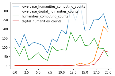
We can see that actually lowercasing words leads to many more matches since all we are doing is trying to match exact patterns and upper and lower case represent differing patterns. While we could use the replace() method for removing punctuation, some of the other approaches listed above require more attention. Let’s dig in!

Lemmatizing/Stemming

Lemmatizing and Stemming are both ways of reducing words to their root form to make them more normalized for analysis. Lemmatizing is the process of reducing words to their base form, while stemming is the process of reducing words to their stem, demonstrated in the figure below:

lemma and stem

The NLTK library we used for FreqDist also comes with stemmers and lemmatizers.

import nltk
from nltk.stem import PorterStemmer
porter = PorterStemmer()

Now to use these we need to apply them to each of the rows in our dataframe. We could do this with a for loop, but it’s more efficient to use the apply() method. To try this out, let’s work on a subset of our humanist_vols dataset.

subset_humanist_vols = humanist_vols[0:2]

def stem_words(row):
    stemmed_words = ''
    for token in row.split(' '):
        stemmed_words += porter.stem(token) + ' '
    return stemmed_words
subset_humanist_vols['stemmed_text'] = subset_humanist_vols.text.apply(stem_words)

print(subset_humanist_vols[0:1]['stemmed_text'].values)

This will print out a large text string with the stemmed words. We can see what the first email looks like when it is stemmed:

from: mccarty@utorepas
subject:
date: 12 may 1987, 23:50:02 edt
x-humanist: vol. 1 num. 1 (1)

thi is test number 1. pleas acknowledge.

And compare it to the original:

From: MCCARTY@UTOREPAS
Subject: 
Date: 12 May 1987, 23:50:02 EDT
X-Humanist: Vol. 1 Num. 1 (1)

This is test number 1. Please acknowledge.

We notice that stemming lowercased the words, but did not remove the punctuation. It also stemmed the words so that there is less variation in the words.

But let’s talk about the code above, and explain how we are doing this. To help make sense of everything, I’ll show the same code written as a for loop below:

stemmed_column = []
for index, row, in subset_humanist_vols.iterrows():
    stemmed_words = ''
    for token in row.text.split(' '):
        stemmed_words += porter.stem(token) + ' '
    stemmed_column.append(stemmed_words)

subset_humanist_vols['stemmed_text'] = stemmed_column

So rather than having a function that takes a row as an argument, we are using a for loop to iterate over the rows. We are first creating an empty variable called stemmed_words and then we are splitting the text column into tokens and then iterating over each token. To do stemming or lemmatizing or many other text analysis methods, you need your words as tokens rather than a giant string. In this example, we are simply splitting on spaces, but there are many other approaches to this problem.

Once we have our tokens we then pass them to the porter.stem() method to stem them. We then append the stemmed words to our stemmed_words variable. Finally we append the all the stemmed words to the stemmed_column variable and then add that back into our dataframe outside of the for loop.

So let’s compare this to our apply method:

def stem_words(row):
    stemmed_words = ''
    for token in row.split(' '):
        stemmed_words += porter.stem(token) + ' '
    return stemmed_words
subset_humanist_vols['stemmed_text'] = subset_humanist_vols.text.apply(stem_words)

Here we have a function called stem_words that takes a row of our dataframe, and then does the similar split to tokens and then stem and assing to stemmed_words. Instead of appending to a list though we are returning stemmed_words on each iteration and assigning it directly to our DataFrame in a new column.

You’ll notice that unlike in our for loop we write row.split() instead of row.text.split(). This is because we are doing the apply directly on the text column. We could also use apply to access all the columns in our dataframe with the following change:

def stem_words(row):
    stemmed_words = ''
    for token in row.text.split(' '):
        stemmed_words += porter.stem(token) + ' '
    return stemmed_words
subset_humanist_vols['stemmed_text'] = subset_humanist_vols.apply(stem_words, axis=1)

In channging subset_humanist_vols.text.apply(stem_words) to subset_humanist_vols.apply(stem_words, axis=1) we are now performing apply on all the columns of the dataframe, row by row. The biggest thing to remember with apply is that you need to pass in the name of the function you want to run into the apply method. You can read more about the apply method https://pandas.pydata.org/docs/reference/api/pandas.DataFrame.apply.html.

Finally you might get an error when you run this code,

SettingWithCopyWarning: 
A value is trying to be set on a copy of a slice from a DataFrame.
Try using .loc[row_indexer,col_indexer] = value instead

See the caveats in the documentation: https://pandas.pydata.org/pandas-docs/stable/user_guide/indexing.html#returning-a-view-versus-a-copy
  subset_humanist_vols['stemmed_text'] = subset_humanist_vols.text.apply(stem_words)

That’s a common Pandas error that has to do with how we’re adding new data to our dataframe. There’s a few different solutions listed here https://stackoverflow.com/questions/20625582/how-to-deal-with-settingwithcopywarning-in-pandas but for ease, I normally just surpress this warning with the following code:

import pandas as pd
pd.options.mode.chained_assignment = None  # default='warn'

Quick Assignment

How might we try and rework our stemming code to work with lemmatizing?

First we’ll need to import the right libraries.

from nltk.stem import WordNetLemmatizer
nltk.download('wordnet')
nltk.download('omw-1.4')
wordnet_lemmatizer = WordNetLemmatizer()

Now try and create a function called lemmatize_words that takes a row as an argument and returns a string of the lemmatized words.

TF-IDF

So far we have been focused on counting and cleaning our textual data, but we could also try some more complex Information Retrieval techniques. One popular approach is an algorithm called Term Frequency - Inverse Document Frequenc or TF-IDF. TF-IDF was first proposed in a 1972 paper by Karen Spärck Jones under the name “term specificity.”

⚡️ Great resources for learning more about TF-IDF are: Matthew J. Lavin, "Analyzing Documents with TF-IDF," Programming Historian 8 (2019) and Melanie Walsh's Textbook

The reason TF-IDF is so popular is because it is intended to surface terms that are distinctive across as set of documents (or a corpus). Often times with word counting you get lots of high frequency words (remember Zipf’s law) but these words aren’t always helpful if you are trying to understand the concepts within the text. High frequency words are more useful for author attribution.

So the way TF-IDF works is the following operations as visualized in this diagram:

tf-idf

To break this down into code it really looks like the following:

term_frequency = number of times a given term appears in document

inverse_document_frequency = log(total number of documents / number of documents with term) + 1*****

tf-idf = term_frequency * inverse_document_frequency

So let’s try it out! We could write this with plain Python, but we can also install the scikit-learn library with the following code pip3 install sklearn. We can then use the code from the Programming Historian lesson linked above to get the following:

# Let's try TF-IDF. This code is from the PH Tutorial linked above
# Import the TfidfVectorizer from sklearn.feature_extraction.text
from sklearn.feature_extraction.text import TfidfVectorizer

#save our texts to a list
documents = subset_humanist_vols.text.tolist()

#Create a vectorizer
vectorizer = TfidfVectorizer(max_df=.7, min_df=1)

The documentation for the TfidfVectorizer is available here https://scikit-learn.org/stable/modules/generated/sklearn.feature_extraction.text.TfidfVectorizer.html and we can see what all these parameters mean. In particular, take a look at max_df and min_df. These parameters control how much frequency a word needs to be in a document to be included in the vocabulary. In our case we want to include words that appear in more than 70% of the documents, but also exclude words that appear in fewer than one document.

Now we need to fit our emails to the vectorizer. We can do this with the following code:

# Fit the vectorizer to our emails
transformed_documents = vectorizer.fit_transform(documents)

# Now get the top features for each document
transformed_documents_as_array = transformed_documents.toarray()

dates = humanist_vols.dates.tolist()
tfidf_results = []
for counter, doc in enumerate(transformed_documents_as_array):
    # construct a dataframe
    tf_idf_tuples = list(zip(vectorizer.get_feature_names(), doc))
    one_doc_as_df = pd.DataFrame.from_records(tf_idf_tuples, columns=['term', 'score']).sort_values(by='score', ascending=False).reset_index(drop=True)
    one_doc_as_df['dates'] = dates[counter]
    tfidf_results.append(one_doc_as_df)

Once that is done we can save our results to a new dataframe and explore the top unique terms

tfidf_df = pd.concat(tfidf_results)
tfidf_df = tfidf_df.sort_values(by=['score'], ascending=False)
tfidf_df.head(10)

You should see a lot of http. To get a better sense of let’s try taking the 200 rows of this tfidf_df but only keeping the unique terms. We can do that with the unique method in Pandas.

print(tfidf_df[0:200].term.unique())

Which should produce this list:

['http' 'utorepas' 'bitnet' 'www' '2007' '2006' '2004' 'gopher' '2005'
 '2002' '2003' 'html' 'ninch' '2008' 'vax' 'uottawa' 'qs' 'prolog'
 'hussein' 'acadvm1' 'kessler' 'doi' 'celia' 'cdt' 'na' '441495' 'cst'
 'penndrls' 'amico' 'brownvm' 'neach' 'epas' 'xxx' '1007' 'fqs' 'tlg'
 'kevitt' 'ocp' 'sanskrit' 'dfl' 'iraq' 'easi' 'pali' 'kleio' 'kurzweil'
 'rahtz' 'cti' 'kentvm' 'bene' 'giampapa' 'hurd' 'htm' 'chiba' 'gas'
 'nota' 'coombs' 'hypercard' 'cont' 'strangelove' 'ubiquity' 'cdn'
 'google' 'vm' 'snobol' 'taunivm' '8080' 'ere' 'ibycus' 'lml' 'koontz'
 'lowercase' 'nicolov' 'mst' 'artfl' 'guvax' 'stallman' 'crosby'
 'germaine' 'ijcai' 'marchand' 'bst'
 '____________________________________________________________________'
 'pst' 'ucs' 'engst' 'aisb' 'israeli' 'mc' 'junger' 'masks' 'iraqi'
 'arundel' '10646' 'nicolas' 'lachance' 'spaeth']

Some of these terms are pretty meaningless and we might want to clean them out, but some like prolog or google look promising. In class, let’s try and compare the tf-idf scores for these terms to the frequency of their counts.