Introduction to Exploratory Data Analysis

⚡️ This lesson is now virtually available below and the notebook used in the video is availble here and from class is available here

Cleaning and Preparing (Text) Data for Exploratory Analyses

We will be working with our Pudding Film Dialogue datasets today. First let’s review some of the concepts we have already covered in our Introduction to Notebooks.

How do we read in our film scripts dataset? How would we sort the values in the dataset? How could we remove all the null values from the dataset? How we group our data by year?

Let’s try out some code together!

So hypothetically we have taken a few minutes to explore and answer these prompts. But besides refreshing our memory for Pandas syntax, we were also doing something called exploratory data analysis and data cleaning.

These are terms you will see a lot in the data science world. But even in digital humanities, we need to both understand our data (think producing a data biography) and often clean it.

So what does it mean to clean data?

The term cleaning data refers to a whole set of transformations that you may or may not decide to undertake. So why would someone clean data? Remember in the “Data Biographies” article by Heather Krause, she discussed subsetting the data to just the data from Rwanda since it was the most consistent across the time period and in its collection - this is a type of data cleaning, in this case selecting a subset of data. Krause made this selection because otherwise there was too much variability in the data quality to perform their analyses.

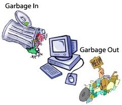
Cleaning data can also mean normalizing distributions, removing null values, and even transforming some of the data to standardize it. But regardless of what you choose to do, the reason to undertake this step is because of the concept of GIGO.

gigo

GIGO stands for “Garbage In, Garbage Out” (to read more about the origins of GIGO, read this article https://www.atlasobscura.com/articles/is-this-the-first-time-anyone-printed-garbage-in-garbage-out). GIGO is important because it essentially means that the quality of your data analysis is always dependent on the quality of your data.

However, for as much as we want to prioritize quality, what are some of the downsides or tradeoffs of cleaning data? Some potential considerations include:

losing the specificity of the original data (especially a danger for historic data but also for data collected by certain institutions)
privileging computational power over data quality or accuracy
releasing datasets publicly without documenting these changes

This list is by no means exhaustive! But number one thing to remember with datasets is that the act of collecting data is in of itself an interpretation. And so cleaning data adds another layer of interpretation (sometimes many layers) to the dataset, which is why its crucial to keep a record of how you transform your data.

It is also important to realize that even with cleaning you will never have a perfect dataset. In humanities data analysis, data cleaning is somewhat controversial because it means distorting the original source material (remember Katie Rawson and Trevor Muñoz, “Against Cleaning”?). So one of the considerations for any humanities data analysis is not only how to data clean, but why and to what degree.

Exploratory Data Analysis with Pandas and Python

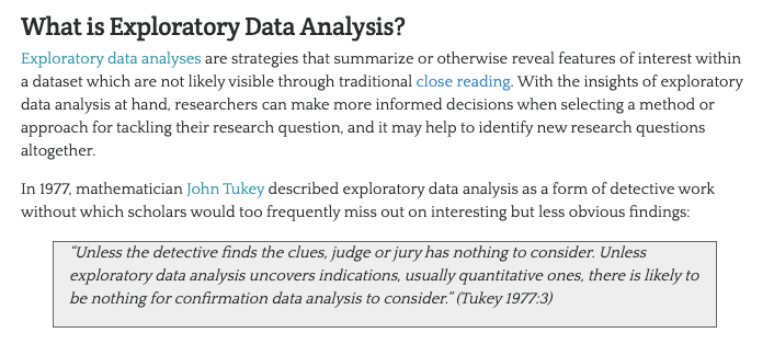
The first step in data cleaning is to not actual clean the data, but instead perform initial exploratory data analysis (EDA) so we can better understand what is there and what isn’t.


From Zoë Wilkinson Saldaña “Sentiment Analysis for Exploratory Data Analysis” https://programminghistorian.org/en/lessons/sentiment-analysis

In his 1977 book Exploratory Data Analysis, Tukey argued that EDA could help suggest hypotheses that could be then tested statistically.

With Pandas we can perform all of the necessary steps for EDA.

We want to explore the data, so we could use head(), tail(), or sample() methods to display a subset of the dataset. We could also use .shape or .dtypes to see shaped of the dataframe and the data types of each column.
Next we might use the describe() method to output a summary of our dataset. According to the documentation for this method, it provides “descriptive statistics include those that summarize the central tendency, dispersion and shape of a dataset’s distribution, excluding NaN values.” (Read the docs here).
After getting this bird’s eye view of the distribution of the data, we could use sort_values() or nsmallest() / nlargest() to either organize the dataset or return the rows with maximum or minimum of values in a certain column.
We can use the isna() to see what values might be missing in the dataset. Remember that isna() can be run on either individual columns or the entire dataframe, and that you can chain it with other methods any() to check if there are any null values in the data.
Finally we would use the plot() method to do some initial graphing of the trends in our data to fully help explore its distribution and potential correlations.

Let’s try this out with our film scripts dataset!

Now once we’ve explore our data, we can start assessing how we might clean the data.

THIS IS AN ITERATIVE PROCESS!

While you might start cleaning your data before undertaking any analyses, it is likely that you will need to re-transform your data many times depending on your methods.

One best practice is to save multiple versions of your dataset as csv files, so that you don’t either overwrite your original data or have to rerun previous transformations.

Remember that with Pandas we can read and write csv files using pd.read_csv() and {name of your dataframe}.to_csv().

Cleaning Data in Pandas

Remember in our movies example we selected a subset of the data using Pandas.

film_scripts[film_scripts.gross_ia >= 0]
film_scripts_cleaned = film_scripts[film_scripts.gross_ia.isna() == False]

You will often want to either drop nulls or select a subset of your data, and you can use the bracket notation in Pandas to select all rows that meet a particular condition. We used to do this with a for loop and we still can in Pandas though it’s not really best practice. Let’s do it anyways!

Copy the following code:

for index, row in film_scripts.iterrows():
    print(index, row)

You should now be seeing a loop that prints out the index and row of each row in the dataframe.

Now let’s try adding in our same conditional logic:

for index, row in film_scripts.iterrows():
    if row.gross_ia >= 0:
        print(index, row)

While this is technically doing the same thing, doing the square brackets to pass in a condition is much faster than using a for loop with Pandas.

Just remember that the syntax always goes dataframe[condition] and that you will need to select the column you want to use your condition on.

We also used groupby to transform our data into new aggregate versions of the data.

films_year = film_scripts_cleaned.groupby('year')
films_year.get_group(2009)

Pandas truly has a massive amount of functionality, so one thing we can do with our films_year is rather than saving it as a pandas.core.groupby.generic.DataFrameGroupBy we can actually save the counts by year into a new column.

films_year = film_scripts_cleaned.groupby('year').size().reset_index(name='counts')
print(films_year)

Now we should see a new column called counts that contains the number of films in each year.

We could also do a similar type of calculation but on a different column in our film_scripts_cleaned dataframe.

film_scripts_cleaned.groupby('year')['gross_ia'].sum().reset_index()

What does this show in your notebook? Try changing the ['gross_ia'] to .gross_ia and see what happens.

You should see it output an identical dataframe. This is because we are using the .groupby() method to group by the year column and then we are specifying a calculation on another column using the .sum() method to sum the gross revenue of films in each of the years.

.sum() is one of many methods that can be used for calculations with a dataframe and you can either use it on the entire dataframe or on a grouped dataframe like we did. See the table below for a few other ones:

Pandas calculations	Explanation
`.count()`	Number of observations
`.sum()`	Sum of observations
`.mean()`	Mean of observations
`.std()`	Standard deviation of observations
`.mode()`	Mode of observations
`.median()`	Median of observations
`.min()`	Minimum of observations
`.max()`	Maximum of observations
`.describe()`	Summary statistics

When exploring your data you might often find duplicates. You can use the drop_duplicates() method on either the entire dataframe or use the subset=[] argument to pass in specific columns. You can also specify which of the duplicates you want to keep (options are the first or last). More information is available in the docs.

You might also want to standardize your data so that you can compare more easily across the dataset.

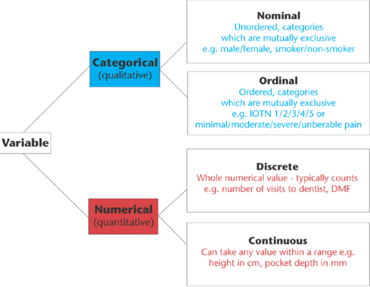
Before you do so, it’s important to have a sense of what types of data exist.

data

This graph outlines the main types of data you might encounter, which largely breaks down between qualitative (categorical) or quantitative (numerical).

For example, say you have gender as a field in your dataset, but who ever initially encoded the data did not do so in a standardize way.

Gender
m
Male
fem.
FemalE
Femle

Before standardizing this data, it’s helpful to consider whether you’re interested in these spelling errors (maybe this is census data for example) or if you want to fix them for your analyses. If you do decide to fix them, they you would be changing the data into categorical and nominal data (rather than categorical and ordinal).

There’s a few ways we could standardize this using Pandas. One is the map() method which takes a dictionary where the keys are the spelling errors and the values are the correct categories.

df['gender'].map({'m': 'male', 'fem.': 'female', ...})

However, say we have quite a few misspellings, it will get tedious trying to write them all out. Instead, we can use pattern matching and regular expressions. Regular expressions (or regex) are any sequence of characters that we can search for in another string. Most programming languages use them and you can learn more about them here https://regexone.com/.

In Python, there is the library re that comes with the Python Standard Library and is built for regex (you can read the docs here https://docs.python.org/3/library/re.html). However, Pandas also has built in functionality for handling regex.

df.gender[df['gender'].str.match(r"m", flags=re.IGNORECASE)] = 'male'
df.gender[df['gender'].str.match(r"f", flags=re.IGNORECASE)] = 'female'

Here we are using the str.match() method and regex to check if the strings in our rows start with these values and are ignoring whether they are upper or lowercase.

Another method is that we could also first lowercase these strings in the gender column and then use the str.contains() method instead.

df.gender = df.gender.str.lower()
df.gender[df.gender.str.contains('fem')] = 'female'
df.gender[df.gender.str.contains('fem') == False] = 'male'

In this example, if we had done str.contains('male') we would have ended up over writing our female values.

Pandas has a number of built in methods for working with strings that can help us check for all sorts of values (like decimals, numbers, or spaces) and transform string values. You can read more about working with text data and pandas here https://pandas.pydata.org/pandas-docs/stable/user_guide/text.html#method-summary.

One final thing to think about though is what might be wrong with our use of gender here? First, gender is not a binary value. We could include more categories to try and capture a broader range of gender identities. However, two important questions to ask in data analysis is whether you actually need this data AND whether this data actually represents what it claims to represent.

Putting It All Together

The final thing we might want to consider is also joining different dataframes together. This is done using the merge() method.

Let’s try taking our groupby dataframe and joining it with the film_scripts_cleaned dataframe.

First we need to save our groupby into a new variable.

films_gross_sum = film_scripts_cleaned.groupby('year')['gross_ia'].sum().reset_index()

Now let’s merge our films_gross_sum dataframe with the film_scripts_cleaned dataframe.

The way we do this is with pandas merge() method. Merging datasets is a very tricky concept that takes time to understand. The Pandas library has very detailed documentation on how you merge datasets https://pandas.pydata.org/docs/user_guide/merging.html. For those familiar with SQL it is a very similar concept, where you can do different types of joins.

merge

This figure shows both the syntax for merging and gives us some visual examples of how to use the merge() method.One thing I recommend is trying to draw out the different steps involved in merging datasets.

We need to think about the different shapes of our dataframes. Try using .shape on the dataframes to see how many rows and columns they have. While we would expect their to be different columns in each dataframe, also pay attention to the number of rows in the films_gross_sum dataframe. When merging dataframes with differing number of rows, we will end up repeating some values which is completely ok but something to think about.
Next we need to decide on our key for merging. A key here is the column that we want to use to join the two dataframes. In this case, we want to join the year column of the films_gross_sum dataframe to the year column of the film_scripts_cleaned dataframe. You can use multiple keys when merging dataframes, and also use the .columns method to get a list of all the columns in a dataframe to see which ones are in common.
Finally we need to decide on how to merge the two dataframes. You’ll notice that merge has a how parameter. This is where we specify the type of join we want to undertake. Below is a graph showing the different types of joins that exist with venn diagrams but the best way to understand this is to do it.

joins

So let’s try merging our dataframes!

# Check columns
print(films_gross_sum.columns), print(film_scripts_cleaned.columns)

Notice anything? We not only have year in common but also gross_ia. However, the value of gross_ia is not the same in both dataframes. So let’s rename the gross_ia column in films_gross_sum to gross_sum. Now we can merge on the year column.

films_gross_sum = films_gross_sum.rename(columns={'gross_ia': 'gross_sum'})
films_gross_sum_merged = pd.merge(films_gross_sum, film_scripts_cleaned, on='year')

We should see now that our dataframes are merged and that for each row there is a gross_sum column, which repeats the year gross sum value. We can experiment with the different how parameters as well, but if you try how='outer' or how='left', and then print out the length of the dataframe you will not see a difference with our current dataframe because of the fact that year does not differ between the dataframes.

That is not true though for the rest of the film dialogue spreadsheets! So be sure to test out different how parameters and see what changes for those dataframes (for example, try merging meta_data7.csv and character_mapping.csv and see how the different how parameters changes the shape of the dataframe).

For more resources on merging dataframes, check out https://www.educative.io/edpresso/three-ways-to-combine-dataframes-in-pandas and for more on Pandas see Melanie Walsh’s https://melaniewalsh.github.io/Intro-Cultural-Analytics/03-Data-Analysis/00-Data-Analysis.html and Jake VanderPlas’s https://jakevdp.github.io/PythonDataScienceHandbook/03.00-introduction-to-pandas.html

We’ve only barely scratched the surface of data cleaning here (for some more examples you can check out https://towardsdatascience.com/the-ultimate-guide-to-data-cleaning-3969843991d4). Nonetheless, you now have some sense of the choices you have to make when cleaning your data and remember that no dataset is ever perfect! The important thing is keeping good records of how you’ve transformed your data and being thoughtful about what your data represents.

Now on to the in-class assignment!