Introduction to Network Analysis
What is a network?
In The Network Turn, we learned that:
The network framework shapes how we interpret the world around us. Nothing is naturally a network; rather, networks are an abstraction into which we squeeze the world. Nevertheless, almost anything can be turned into a network, whether it be the interactions between characters in Shakespeare’s plays, the dissemination of memes on Facebook, or the trade network implicated in the ancient Roman brick industry.
But what is a network exactly?

We discussed this figure below in class and how we have things called nodes and edges in a network, but we didn’t get a chance to actually talk through how you take cultural data and turn it into a network.
In The Network Turn Chapter 5, the authors discuss taking correspondence letters and transforming them into networks, using the following information:
- John Smith wrote to Peter Jones three times: on 3 January 1596, 21 March 1596, and 12 December 1597.
- Peter Jones wrote to John Smith once: on 4 February 1596.
- John Smith wrote to Mary Smith twice: on 15 May 1596 and 25 July 1597.
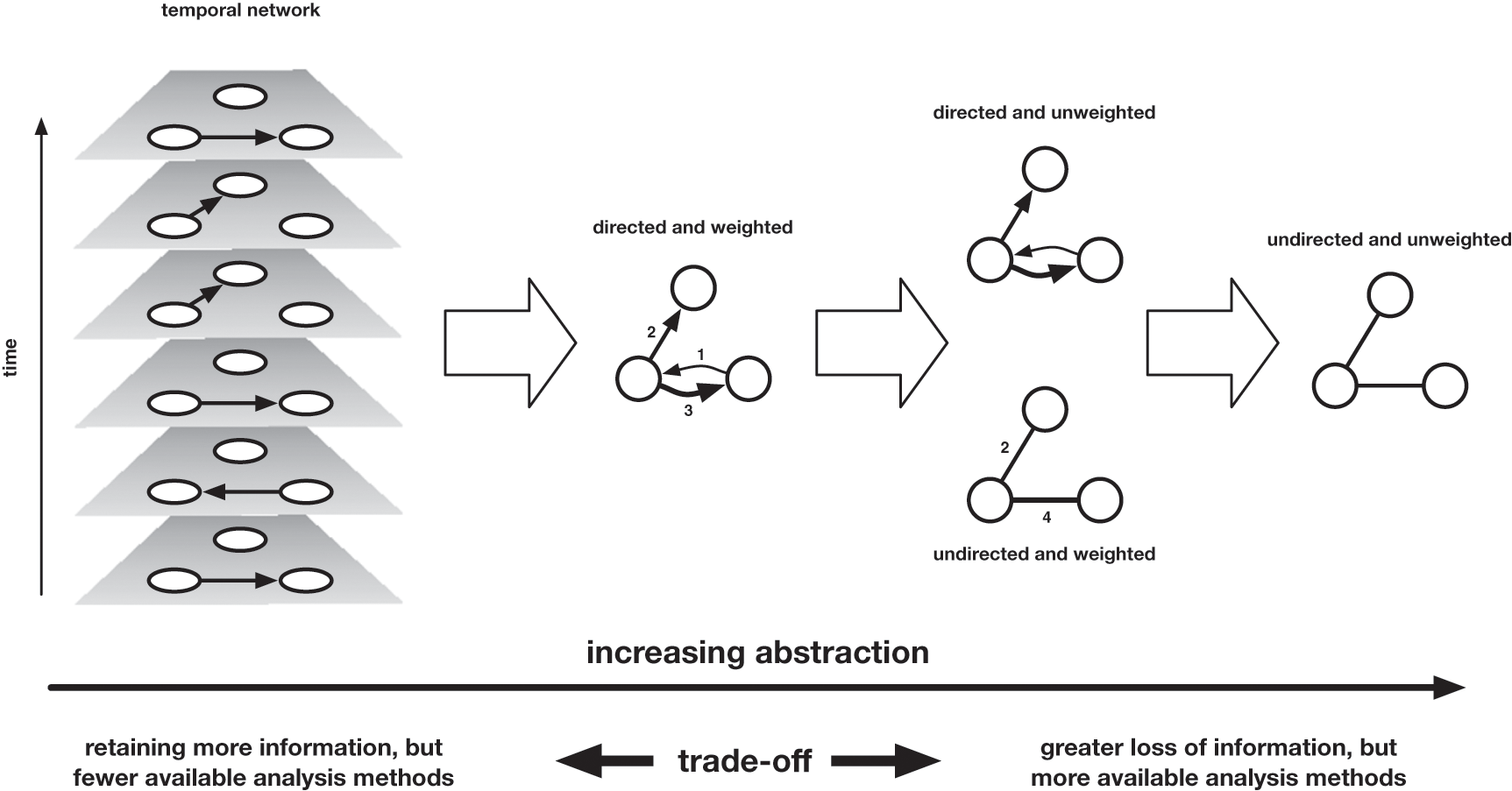
The authors discuss how you can represent this data as networked data with the following figure:

They discuss how if you assume that the individuals are nodes, then you have to decide what information to use to reprsent edges.
Moving from left to right, we move across a landscape of abstraction, which entails more information loss the further we travel. The rightmost representation of the network merely records the existence of an edge between these nodes, without any attention to the time at which these edges formed, the direction in which letters travelled (who was the sender, who the recipient), or the volume of correspondence that travelled along those edges. One step less abstract is the directed network, which records the direction in which letters travelled (but not the volume), and the weighted network, which encodes the volume of correspondence that marks those edges (but not the direction). One further step leftward is the weighted and directed network, which combines the two previous network attributes, Finally, the leftmost network is a temporal network, which records the direction and time of every item of correspondence separately.
While it might seem obvious to choose the network that most accurately represents these letters, the authors discuss how this version provides the least amount of algorithmic power. So when creating networks from cultural data we need to balance this question of accurately representing our materials with wanting to leverage the power of computation.
Networks from Cultural Data
So let’s try out building a network from our data to get a sense of these tradeoffs.
On Tuesday we stopped short of retraining our NER model, so let’s re-open our IntroNER notebook and finish that task.
We stopped after merging our datasets so the next step is to try and get a list of the characters that The Pudding identified so that we can improve our NER model.
One thing to note is that I changed our sample film script from Kill Bill to Twilight so that we have a few more named characters in our dataset.
So in our notebook how could we get a list of all the identified characters that appear in Twilight?
## Get a list of all the identified characters
Now that we have this list we can start fine tuning our NER model. In our Intro to NER, I had some code that showed how you could refine the NER pipeline to get a better result. I’ve rewritten that code to work with our list and let’s take a look at in our Jupyter notebook.
list_names = [{"label": "PERSON", "pattern": [{"LOWER": f"{name}"}], "id": f"{name}"} for name in identified_chars if len(name.split(' ')) == 1]
list_full_names = [{"label": "PERSON", "pattern": [{"LOWER": f"{name.split(' ')[0]}"}, {"LOWER": f"{name.split(' ')[1]}"}], "id": f"{'-'.join(name.split(' '))}"} for name in identified_chars if len(name.split(' ')) > 1]

all_names = list_names + list_full_names
print('example rule', all_names[0])
So now we need to pass this list to our spaCy model. We can either train a blank model from scratch or retrain an existing model.
full_nlp = spacy.load("en_core_web_sm")
ruler = full_nlp.add_pipe("entity_ruler")
ruler.add_patterns(all_names)
Now let’s tweak our existing get_entities function to use our new NER model and save our output to a new column improved_identified_characters.
Now that we have our characters identified, we need to consider how would we represent this data as a network? We need to decide what to represent as nodes and edges.
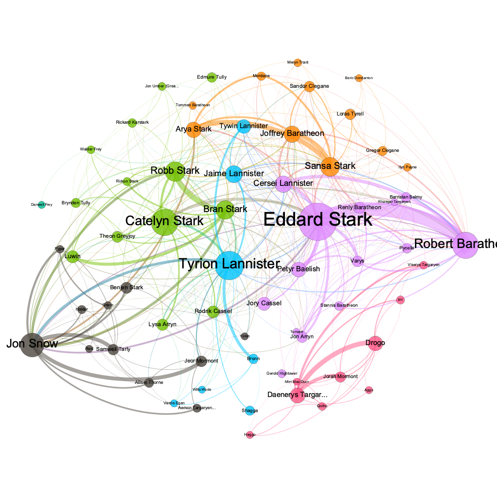
One example that is popular in network science is the Game of Thrones network. Melanie Walsh uses it in her network analysis lesson available here.

Going to the original paper, “Network of Thrones” by Andrew Beveridge and Jie Shan, we can explore how they created this dataset. We can also see the dataset here https://github.com/melaniewalsh/sample-social-network-datasets/tree/master/sample-datasets/game-of-thrones.
So what are the sources for this dataset? And how was it transformed into a network?
We parsed the ebook, incrementing the edge weight between two characters when their names (or nicknames) appeared within 15 words of one another. Afterward, we performed some manual validation and cleaning. Note that an edge between two characters doesn’t necessarily mean that they are friends—it simply means that they interact, speak of one another, or are mentioned together.
We can see from this description that the authors are making some interpretative choices for how to turn prose into networked data. What are some other ways we might consider creating this dataset?
In Class Assignment
Working with our scripts dataset and in groups discuss how you might parse the data and turn it into a network. Even if you have never seen this particular film, what might be an interesting interaction similar to the Game of Thrones example?
Once you’ve decided how you want to represent the connections between characters, try writing some code to take the Twilight film script and count the times characters co-occur in the script.
You might want to try out the sent_tokenize function from NLTK to split the script into sentences. Or write your own function to split the script into chunks.
Then you will need to find all the instances of the characters in each of those chunks and count the number of times they co-occur.
Advanced Networks
From our in class exercise, we now are starting to get a sense of how much work is required to actually take this unstructured data and turn into the shape we need.
Depending on how far groups get, we will either share group code or we will work together over Zoom.
Ideally we we will end up with a dataset that has two-three columns source, target, and weight.
I have already created these datasets, and the weighted Twilight network is available here and the unweighted version is available here.
Now we can start working with this data as a network. To so, we will need to use the networkx library.
import networkx as nx
Since our data is in a DataFrame, we are going to create our network using the from_pandas_edgelist function.
df = pd.read_csv('weighted_twilight_network.csv')
G = nx.from_pandas_edgelist(df,, source='source', target='target', edge_attr='weight')
Now we can start to inspect our network.
G.nodes(data=True)
G.edges(data=True)
We won’t get into depth on network metrics here, but we can very quickly see that Networkx has a lot of different functions that we can use to get a sense of the network.
nx.degree(G)
nx.betweenness_centrality(G)
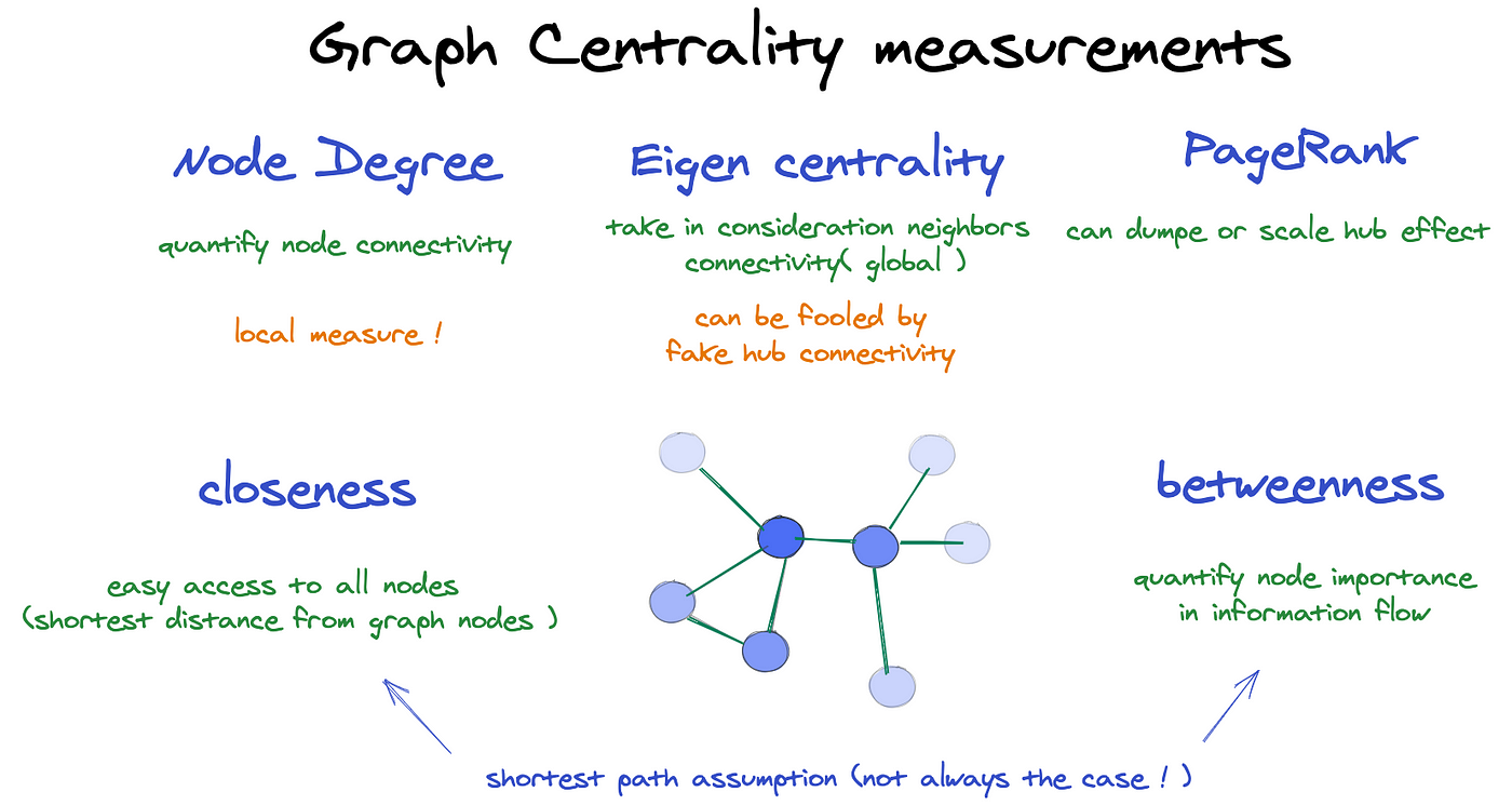
These two functions calculate two very popular network metrics, degree and betweenness_centrality. These are but two of many centrality measures:

And returning to The Network Turn, we can start to get a sense of what these are calculating and what they might mean for our network.
“An extremely simple network measure is a node’s ‘degree’, which is the total number of connections it has with other nodes. […]While the degree of a node is a fundamental measure for the analysis and comprehension of networks, it is also a fairly blunt instrument. However, numerous other ‘centrality’ measures use global properties of the network to help us understand the local significance of a node in interesting ways, such as closeness centrality, betweenness centrality, eigenvector centrality, and PageRank. As the name suggests, closeness centrality defines the centrality in terms of its distance to all other nodes. The peripherality of a node is defined as the sum of its distances from all other nodes; the ‘closeness’ is the inverse of this equation. Closeness can therefore be regarded as a measure of how long it will take to spread information from a given node to all other nodes sequentially. Linton Freeman first quantitatively defined betweenness centrality as the fraction of shortest paths between any two nodes in the network that passes through a given node or edge (Reference FreemanFreeman, 1977).Footnote10 For this reason, betweenness has been used to think quantitatively about the influence a node may have on the flow of information across the network. Following the emergence of large-scale computational network analysis, betweenness can now be calculated efficiently for large networks and can be used, for example, to find effective ways to fragment a network into disjoint components, and to identify modules, or ‘communities’ in the network.”
Visualizing our Network
Let’s try out some ways to visualize our network:
- Networkx and matplotlib https://networkx.org/documentation/stable/auto_examples/index.html
- Pyvis https://pyvis.readthedocs.io/en/latest/
- Palladio http://hdlab.stanford.edu/palladio/
- Network Navigator https://networknavigator.jrladd.com/
- RawGraphs https://rawgraphs.io/
- Network Altair https://github.com/Zsailer/nx_altair
Further Resources
- Networkx Tutorial https://networkx.org/documentation/stable/tutorial.html
- ProgrammingHistorian Tutorial on Networks https://programminghistorian.org/en/lessons/exploring-and-analyzing-network-data-with-python
- Melanie Walsh’s tutorial mentioned above https://melaniewalsh.github.io/Intro-Cultural-Analytics/06-Network-Analysis/01-Network-Analysis.html