(Re)Introduction to Jupyter Notebooks & Pandas
So far in the course, when we’ve been writing Python code, we’ve either been using the Python interpreter in the terminal or saving a Python script. However, there’s a third way to write Python code that’s very popular - that is with Jupyter notebooks.
So what is a Jupyter notebook?
Jupyter notebooks are a type of computational notebook, which is a type of document that can contain both code and rich text elements, such as figures, images, links, equations, and more. When you run code in a Jupyter notebook, the results appear directly beneath the code. This makes it a great tool for data analysis and visualization.
So rather than writing a script and running it, you can write code in a Jupyter notebook and then run the cell to see the results. This is particularly useful for data analysis and debugging, as you can see the results of your code immediately.
Some people even use Jupyter notebooks to publish books and articles. For example, Melanie Walsh’s textbook Introduction to Cultural Analytics & Python is a collection of Jupyter notebooks, combined into a Jupyter book (you can explore the code in this GitHub repository: https://github.com/melaniewalsh/Intro-Cultural-Analytics). Another great example is the Journal of Digital History, which publishes Jupyter notebooks as articles (you can explore their articles here: https://journalofdigitalhistory.org/).

Getting Started with Jupyter Notebooks
The first step to trying out Jupyter notebooks is to install Jupyter. We can install Jupyter with pip (fyi if you are using anaconda, you already have Jupyter installed).
First, we need to activate our virtual environment. If you haven’t already, navigate to the directory where your virtual environment is located and activate it, running the following command if you’re on a Linux/Unix/MacOS system:
source is310-env/bin/activate
Or if you are using a Windows system, you can run the following command for Command Prompt:
is310-env\Scripts\activate
Or for PowerShell:
.\is310-env\Scripts\Activate.ps1
Remember to use the exact name of your virtual environment, if you did not name it is31-env
Now we need to install Jupyter. We can do this with the following command:
pip install jupyter
Since we are using a virtual environment, we’ll also need a few extra commands:
pip3 install ipykernel
python3 -m ipykernel install --user --name=is310-venv
This will make it so that your Jupyter notebook can access our virtual environment (i.e. it knows where your Python libraries are).
Jupyter Notebooks in the Browser
Once everything is installed, we can start a Jupyter notebook by running the following command in our terminal (would recommend doing this in your is310-coding-assignments directory):
jupyter notebook
This command immediately opens the Jupyter interface in our browser, usually at the following address: http://localhost:8888/tree. If it doesn’t open automatically, you can copy and paste this address into your browser.
Localhost is a special name that refers to the computer you are on. So when you open a Jupyter notebook, you are opening a server on your computer that is running the Jupyter notebook interface. This is why you can only access the notebook from the computer it is running on and can’t just send someone a link to your notebook.
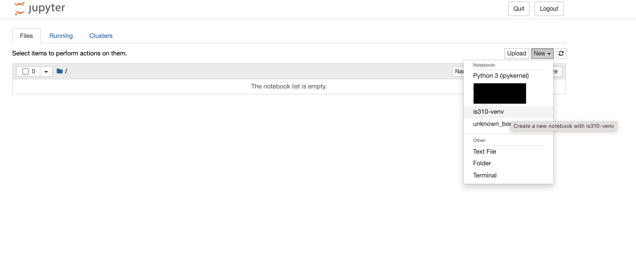
Our first step is to create a new Python 3 notebook using the new button. You’ll notice that when you select new, you have the option to create a new Python 3 notebook or to use a virtual environment. We want to create a new notebook with our is310-env virtual environment so that we have access to all the libraries we’ve installed.
This opens up an empty notebook. You’ll notice that on the right hand side there’s a box that says Trusted and then next to that is the name of our virtual environment. This means that our notebook is running in our virtual environment. If you want to change this, you can select the Kernel dropdown menu and select a different virtual environment.
Now currently our notebook is named Untitled, but if we click on that name we can rename it.
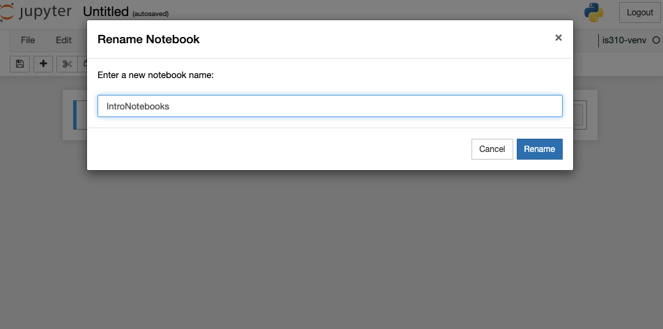
I renamed my notebook IntroNotebooks (generally Jupyter notebooks are named using camel case, but you can name them whatever you want). Jupyter notebook autosaves your notebook, but it is always a good idea to explicitly save it, which you can do by clicking on File and then Save and Checkpoint, or by clicking the save icon in the toolbar (it is the floppy disk icon 💾).
Now when you look at your directory, you should see a new file called IntroNotebooks.ipynb. This is your Jupyter notebook file. Notice the extension .ipynb - this is the file extension for Jupyter notebooks.
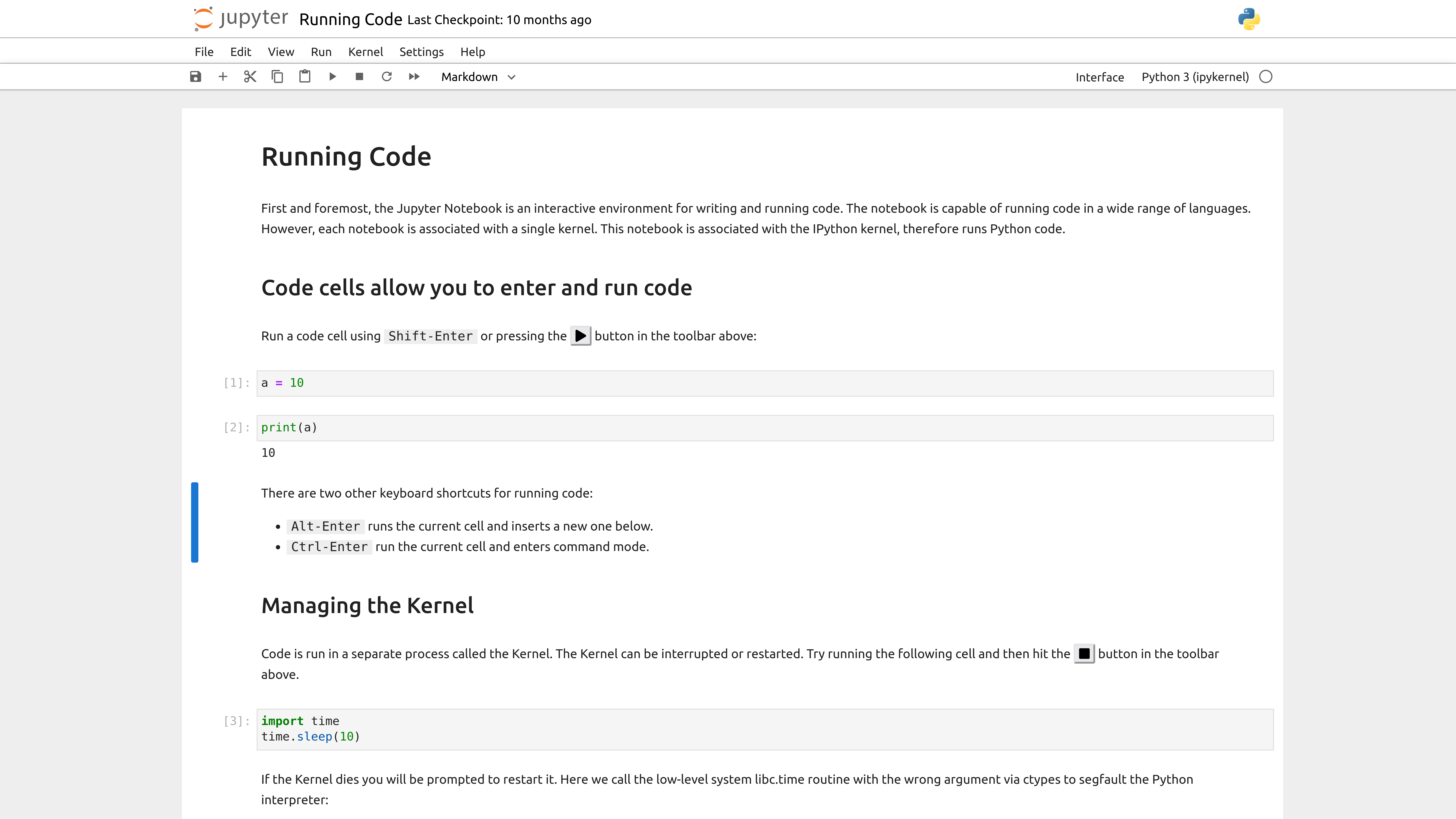
Just like in the terminal, there are shortcuts we can use for working with Jupyter notebooks.
| Mac | Jupyter Function | Windows |
|---|---|---|
Shift + Return |
Run cell (Both modes) | Shift + Enter |
Option + Return |
Create new cell below (Both modes) | Alt + Enter |
B |
Create new cell below (Command mode) | B |
A |
Create new cell above (Command mode) | A |
D + D |
Delete cell (Command mode) | D + D |
Z |
Undo cell action (Command mode) | Z |
Shift + M |
Merge cells (Command mode) | Shift + m |
Control + Shift + - |
Split cell into two cells (Edit mode) | Control + Shift + - |
Tab |
Autocomplete file/variable/function name (Edit mode) | Tab |
Jupyter Notebooks in VS Code
While we can run our notebooks in the browser, we can also run them in VS Code. The benefit to running them in VS Code is that we can use the same interface for writing code and running notebooks, and we can take advantage of the other features of VS Code, such as the debugger, autocomplete, and GitHub Co-Pilot.
First, we should stop the Jupyter notebook server, which you can do by either pressing the Quit button on the main page or type Ctrl+c in the terminal and confirming by typing y and pressing enter. Then we can open VS Code and navigate to the directory where our notebook is located. You can either open the file only or open the entire directory.
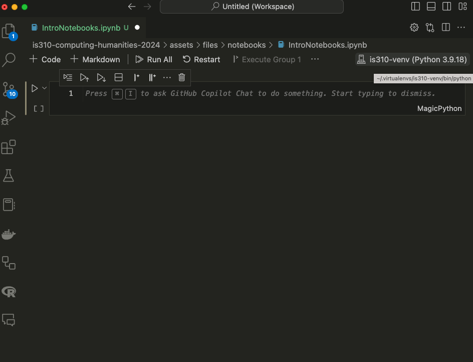
Once you have your notebook open, you’ll again see a Select Kernel option in the top right corner. You can select your virtual environment from this dropdown menu. And if you want, you can create a new notebook entirely in VS Code by pressing ctrl + shift + p and then typing Jupyter: Create New Blank Notebook.
And finally to save your notebook, you can press ctrl + s or go to File and then Save.
Writing Code & Markdown in Jupyter Notebooks
Now that we have our notebook, we can start writing some code. Jupyter notebooks have two types of cells: code cells and markdown cells.
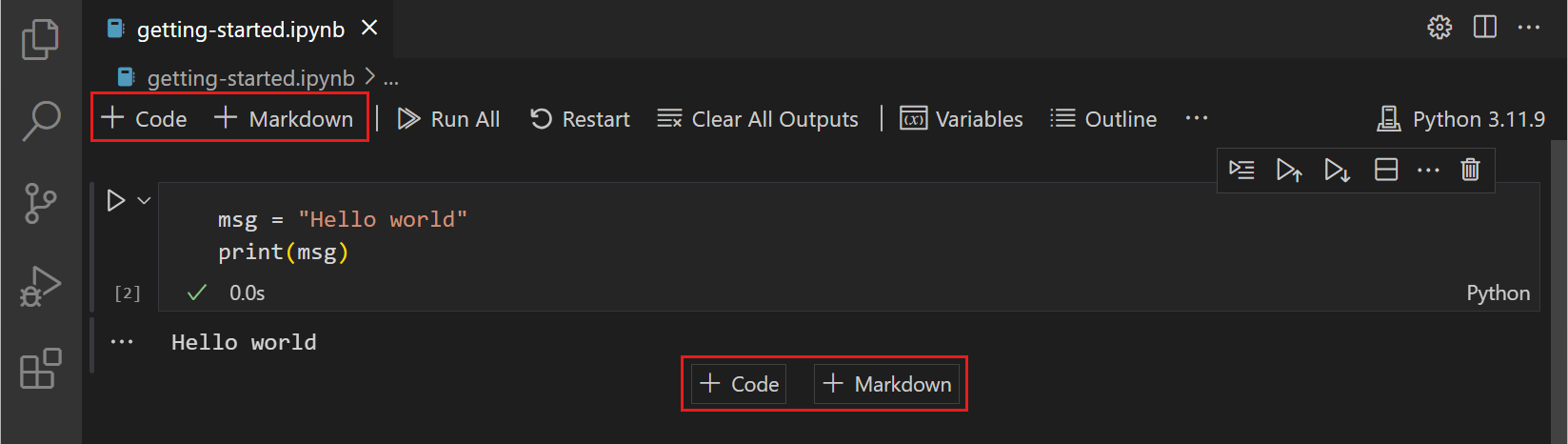
Initially, the notebook will create a code cell, which is where we can write Python code. We can also change the type of cell by clicking on the cell and then selecting the type from the dropdown menu in the toolbar. We can also hover at the top or bottom of the cell and that will display a + Code or + Markdown button.
Let’s first add our title to the notebook, by hovering at the top and selecting + Markdown cell. That will create a new cell above the existing one Then type # Introduction to Jupyter Notebooks and press Shift + Return on a Mac or Shift + Enter on Windows to run the cell.

Now we should see the title at the top. We can use any of the Markdown syntax we have learned so far to format our text. For example, we can use ## for a subheading, * for italics, ** for bold, and --- for a horizontal line, etc.
Now in a Jupyter notebook, we can still use much of the same Python syntax as our scripts. For example, going back to our Complex Python lesson, we could reuse some of the same code in this notebook (though I did add a few tweaks).
Try pasting the following within the first cell of the Jupyter notebook:
def check_movie_release(movie):
    if movie['release_year'] < 2000:
        print(f"{movie['name']} was released before 2000")
    else:
        print(f"{movie['name']} was released after 2000")
        return movie['name']

recent_movies = []

favorite_movies =[
    {
        "name": "The Matrix IV",
        "release_year": 2022,
        "sequels": ["The Matrix I", "The Matrix II", "The Matrix III"]
    },
    {
        "name": "Star Wars IV",
        "release_year": 1977,
        "sequels": ["Star Wars V", "Star Wars VI", "Star Wars VII", "Star Wars VIII", "Star Wars IX"],
        "prequels": ["Star Wars I", "Star Wars II", "Star Wars III"]
    },
    {
        "name": "The Lord of the Rings: The Fellowship of the Ring",
        "release_year": 2001,
        "sequels": ["The Two Towers", "The Return of the King"]
    }
]

for movie in favorite_movies:
    result = check_movie_release(movie)
    if result is not None:
        recent_movies.append(result)

print(recent_movies)
Unlike with our scripts where we would need to save our file and then type python3 script.py, we can just click on the cell and either press Shift + Return on a Mac or Shift + Enter on Windows to run the cell.
Once you run the cell, you should see the following:
['The Matrix IV', 'The Lord of the Rings: The Fellowship of the Ring']
You’ll notice that now there’s a number next to the cell. That indicates the order in which the cells were run. If you run a cell again, the number will increase. This is useful for keeping track of the order in which cells were run, especially if you have a large notebook.
Unlike with scripts, notebooks hold variables in memory, which means that our function now exists in the notebook and we can call in a new cell.
To test this out, add a new cell below our function one by pressing the + Code symbol when you hover. Then paste the following code and run it.
def updated_check_movie_release(movie, released_after_year, released_before_year=2024):
    if released_after_year < movie['release_year'] and movie['release_year'] < released_before_year:
        movie['recent'] = True
    else:
        movie['recent'] = False
    return movie
Now we can call this function in our for-loop by updating the original code:
for movie in favorite_movies:
    updated_movie = updated_check_movie_release(movie, 2020)
    if updated_movie['recent']:
        recent_movies.append(updated_movie['name'])
Now we should see just the The Matrix IV in our list of recent movies. You’ll notice I didn’t have to move the new function above our for-loop. But what happens if I save and close, then reopen the notebook?
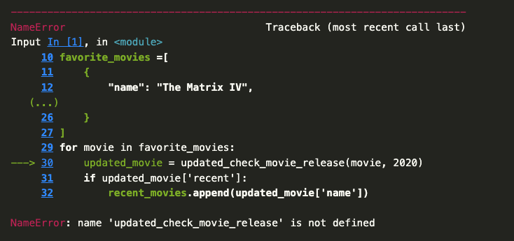
You’ll notice that we get a NameError when we try to run the cell. This is because the function updated_check_movie_release is no longer in memory. This is one of the things that makes Jupyter notebooks great to use, but easy to mess up. We can run cells in any order, which means that we can easily lose track of what’s in memory. So to fix our mistake, we would need to move the updated function before we call it in the for-loop.
Data in Jupyter Notebooks
Jupyter notebooks are particularly useful for working with tabular data (that is data in spreadsheets), especially with a custom-Python Library called pandas. We have already seen pandas in action last week, but let’s try it out in our Jupyter notebook.
First we need to install pandas using either pip install pandas or pip3 install pandas. If you are using a virtual environment, make sure it is activated before you install pandas.
Then we can import pandas into our notebook by typing import pandas as pd in a cell and running it.
import pandas as pd
Remember the as keyword is used to give a library a nickname, so that we don’t have to type pandas each time we want to use a feature of the library. We can check that this worked, by outputting the version of Pandas, with the following:
pd.__version__
Now we’re going to try reading in some tabular data (aka a spreadsheet) into our notebook. So far, we’ve already worked with one in our web scraping assignment, so let’s reuse the same “Film Dialogue” by The Pudding data (that is available here). Be sure to move the downloaded file within the same folder as your Jupyter notebook.
Once we have this file, we can read it into our notebook so that we can access the data using the built-in method from pandas called read_csv().
Paste the following code into a new cell:
film_scripts = pd.read_csv('cleaned_pudding_data.csv')
Before we explore the variable film_scripts, we can also learn a bit more about read_csv(), using Pandas built-in help() method.
Below film_scripts, paste:
help(pd.read_csv)
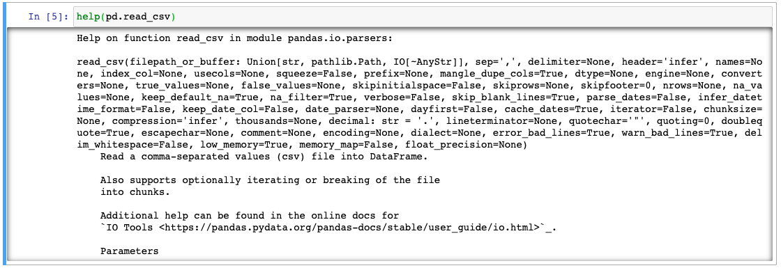
help() is a built-in Python method that provides documentation for a particular function. In this case, it tells us that read_csv() is a method that reads a comma-separated values (csv) file into a DataFrame. It also tells us that we can pass a number of arguments to read_csv(), such as sep (which is the delimiter to use), header (which is the row to use as the column names), and names (which is a list of column names to use). Alternatively, we can always use the Pandas documentation https://pandas.pydata.org/pandas-docs/stable/reference/api/pandas.read_csv.html.
So now let’s inspect film_scripts.
First, we can test what the variable contains by using type(film_scripts), which tells us that it a pandas.core.frame.DataFrame. Notice how we aren’t using the print() method here, but rather just typing the variable name and running the cell. That’s because Jupyter notebooks will automatically print the output of the last line of a cell.
help(pd.read_csv)
type(film_scripts)
DataFrames are the primary data structures in pandas (think like dictionaries or lists, though it is technically a DataFrame class) and are defined as: “a 2-dimensional labeled data structure with columns of potentially different types. You can think of it like a spreadsheet or SQL table, or a dict of Series objects.” You can read more about them here https://pandas.pydata.org/pandas-docs/stable/getting_started/dsintro.html#dataframe

We can then display the data in the DataFrame a few different ways.
First, we can type the variable film_scripts into a cell, which shows us the columns and a few rows, though much of the DataFrame is truncated.
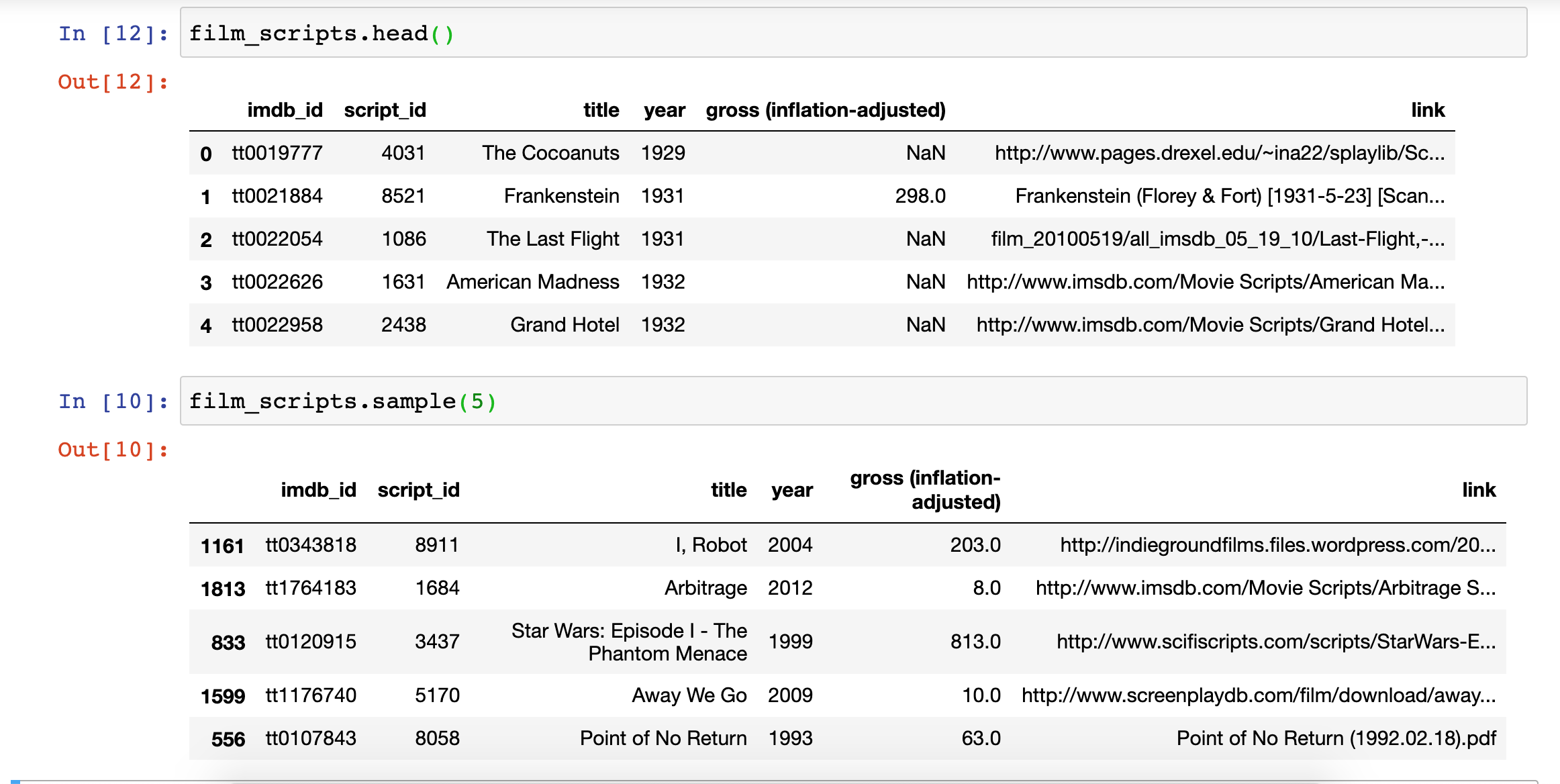
We can also type film_scripts.head(), which prints out the first few rows or film_scripts.sample() which prints out a random sample of rows.
We might also want to explore the size of our dataset, as well as the types of data it contains.
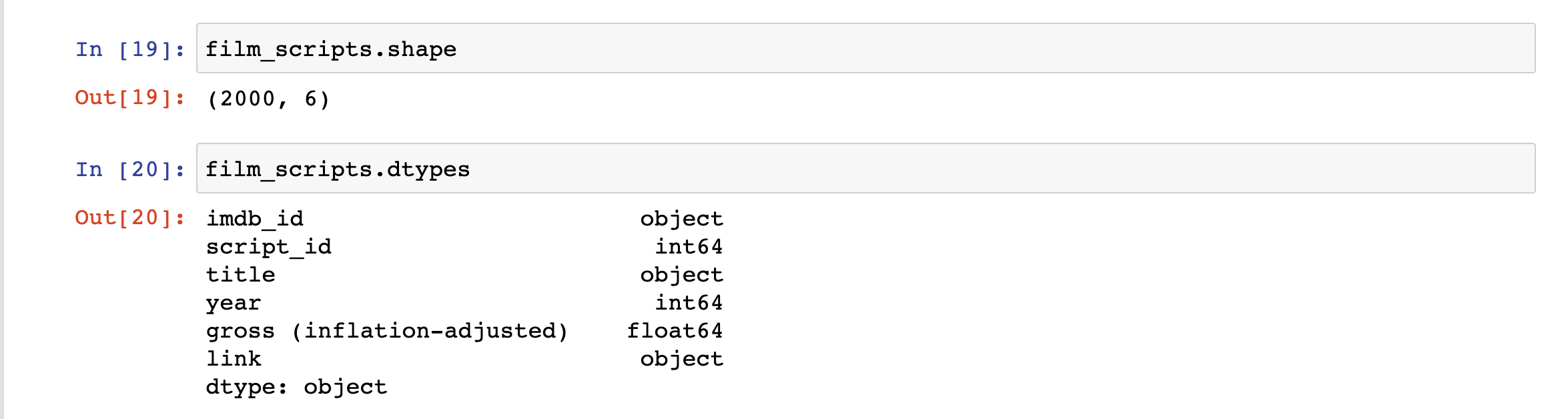
We can use the shape and dtypes attributes that are built-in on the DataFrame Class. shape tells us that we have a certain number of rows and columns, while dtypes tells us the data types of each of those columns.
Pandas data types build from ones available in Python. This tables compares Pandas to Python and another library called numpy (you read more about Pandas data types from here).
| Pandas dtype | Python type | NumPy type | Usage |
|---|---|---|---|
| object | str or mixed | string_, unicode_, mixed types | Text or mixed numeric and non-numeric values |
| int64 | int | int_, int8, int16, int32, int64, uint8, uint16, uint32, uint64 | Integer numbers |
| float64 | float | float_, float16, float32, float64 | Floating point numbers |
| bool | bool | bool_ | True/False values |
| datetime64 | NA | datetime64[ns] | Date and time values |
| timedelta[ns] | NA | NA | Differences between two datetimes |
| category | NA | NA | Finite list of text values |
You’ll notice that some of the data types are only available in Pandas. It’s important to check what data types exist in your columns, since it informs the types of data manipulation you can do with your dataset.
Let’s explore the link column. To access a particular column in Pandas, we can use a few different syntaxes. Try typing in one cell film_scripts['link'] and then in the following cell fiml_scripts[['link]]. What differences do you notice?
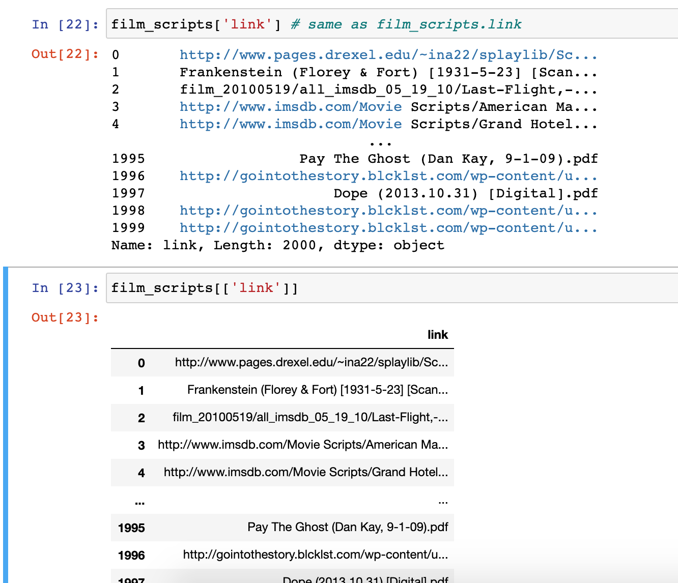
The difference in the output for each of these syntaxes has to do with how Pandas handles indexing (as a refresher, we index in Python using single square brackets).
In Pandas, using a single bracket is used to index either a single column or selected rows, and essentially refers to one dimension of the DataFrame (rather than two). Whereas two square brackets allows us to both index for a column, but then also potentially request a list of columns.
Let’s try out some examples:
- Type
film_scripts[0:5]in a cell and run it. What results do you get? - Type
film_scripts[['link', 'title']]in a cell and run it. What results do you get?
For the first example, you should see the first five rows of the DataFrame, while the second example should show you the data in the columns link and title.
To understand the difference between these types of indexing, we can type following:
print(type(film_scripts['link']))
print(type(film_scripts[['link']]))
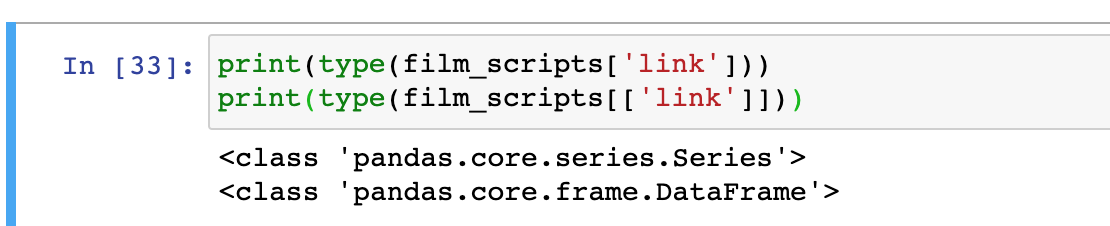
The output here tells us that the first example is returning a class type Series, while the second example is returning a class type DataFrame. While DataFrames are two-dimensional data structures, in Pandas, Series are used to store one-dimensional data (like a column). You can learn more about indexing from the Pandas documentation https://pandas.pydata.org/pandas-docs/stable/user_guide/indexing.html.
Let’s start exploring the data in the link column. Try typing:
film_scripts['link'].tolist()
You should get a long list of all the values in the column as your output. Notice that while some of the items are .html pages, others are .txt files. Someone coming to this dataset might assume that link represents only .html pages, so how can we provide a better column name?
Let’s use pandas rename() method to rename our column. We can read the documentation here https://pandas.pydata.org/pandas-docs/stable/reference/api/pandas.DataFrame.rename.html
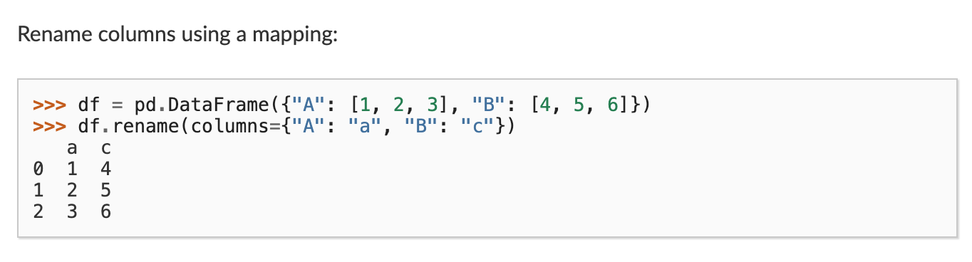
Looking at the documentation we can see that we call rename() after our DataFrame and pass it an argument called columns which takes a dictionary of old column names as keys and new column names as values.
So let’s try it out:
film_scripts.rename(columns={'link': 'source'})
However one issue with this code is that if we use film_scripts in a new cell, it won’t show this new column name. To save our result we need to use the inplace argument in rename.
film_scripts.rename(columns={'link': 'source'}, inplace=True)
Now when we run this cell, film_scripts will contain the updated column name (unless we reload the data into the notebook and overwrite film_scripts).
Instead of renaming the column, we could have also copied the column into a new one that we add to the DataFrame.
Try out:
film_scripts['link'] = film_scripts['source']
Now we’ve recreated our link column, which defeats our purposes. So we can also delete a column using Pandas drop() functionality.
Paste:
film_scripts_dropped = film_scripts.drop(['link'], axis=1)
In this case, we assigned a copy of the DataFrame film_scripts to a new variable called film_scripts_dropped and then also dropped the column link. Just like with standard Python syntax, we can assign DataFrames to new variables depending on how we want to store and manipulate our data.
With Pandas we can also manipulate the DataFrame organization based on the data within the rows.
For example, if we want to see the data organized by title alphabetically, we could use the sort_values() method.
film_scripts.sort_values(by=['title'])
Now we can see that the first movie alphabetically was actually “(500) Days of Summer.”
Try putting in film_scripts.columns in a cell and running it.
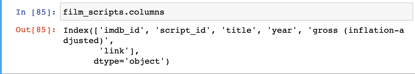
.columns outputs the names of all the columns in the DataFrame.
Let’s rename 'gross (inflation-adjusted)' into something that’s easier to type, like gross_ia. When we index the DataFrame to select gross_ia as a column, what is in the data value in the first cell?
The output of film_scripts[['gross_ia']] should be NaN. This stands for “Not a Number” and is Pandas’ way of telling us that there’s no data in the first row for this column.
Pandas has great documentation for dealing with missing data that you can read here https://pandas.pydata.org/pandas-docs/stable/user_guide/missing_data.html.
We’ll focus on using filtering to remove this missing data. One of the easiest ways we can filter is simply seeing how many of the values are equal to or above zero.
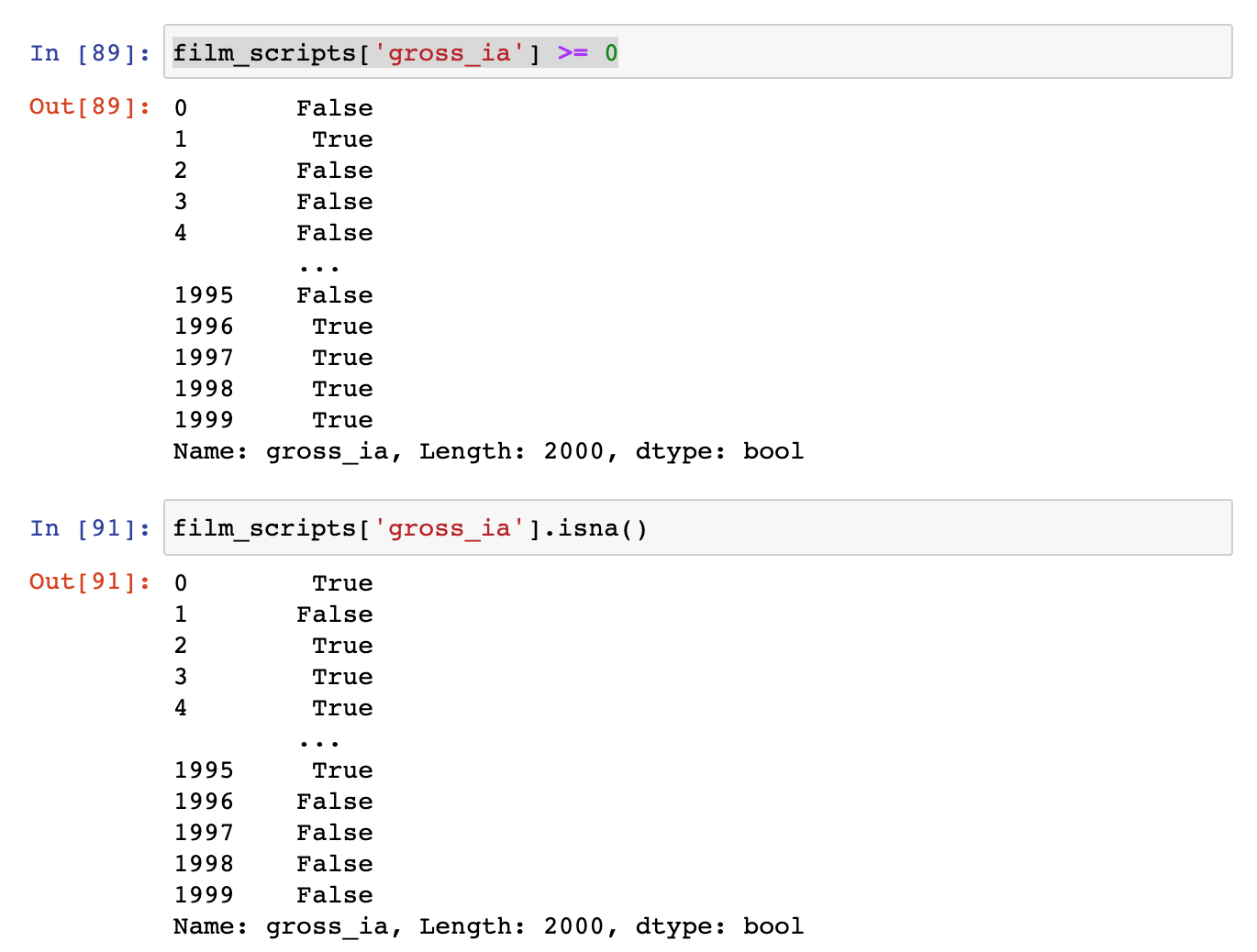
You’ll notice that we can use a conditional expression with the gross_ia column to tell us which cells are empty (hint False here would indicate that the cell contains NaN). We can also use the built-in isna() method which will check if any of the cells are empty and return True if they are.
Now if we want to remove all the rows with empty values for gross_ia, we can simply filter the DataFrame using the following code.
film_scripts[film_scripts.gross_ia >= 0]
Now rather than two thousands rows, we have a DataFrame with 82 rows.
We can save this into a new variable:
film_scripts_cleaned = film_scripts[film_scripts.gross_ia.isna() == False]
And now start calculating some summary values for the DataFrame.
For example, we could calculate the total gross income for all the films using the sum() method.
film_scripts_cleaned.gross_ia.sum()
This gives us the value of 11694.0, which might be interesting but is likely too much aggregation of our data to be useful.
One question we might have is how much gross happened per year in this dataset? How would we start answering this question?
One thing we do is try and find out how many movies are recorded for each year, using the value_counts method. This method counts the unique values in each column https://pandas.pydata.org/pandas-docs/stable/reference/api/pandas.Series.value_counts.html
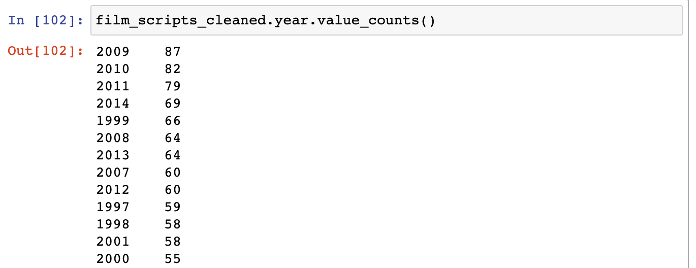
This shows us that years with the top amount of films were 1992 and 1997. However, this doesn’t really tell us how much total gross exists for each year.
To calculate that we need to group together the rows by their years and then add together the values in gross_ia.
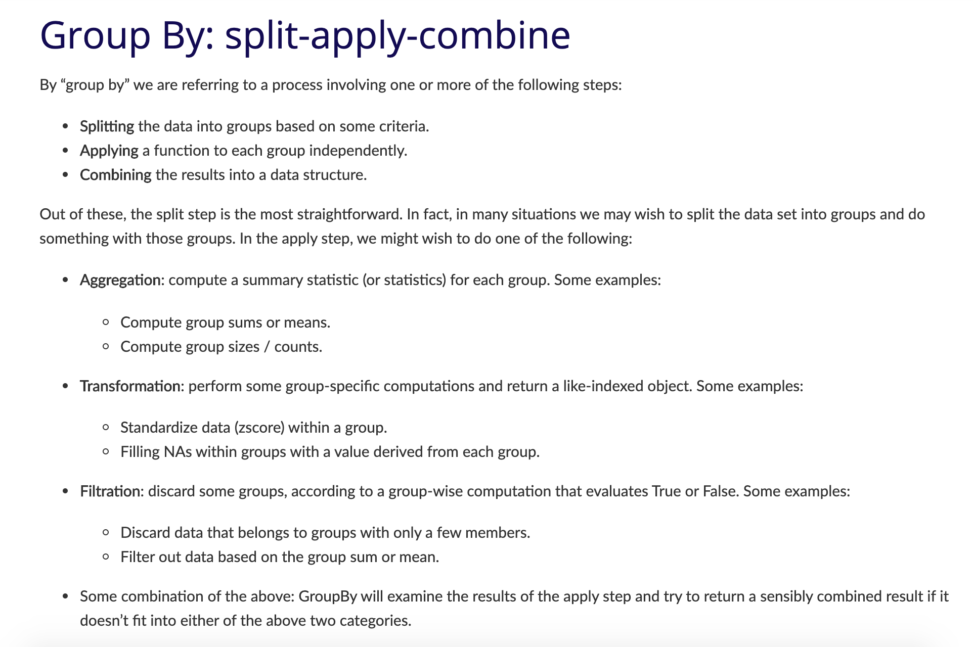
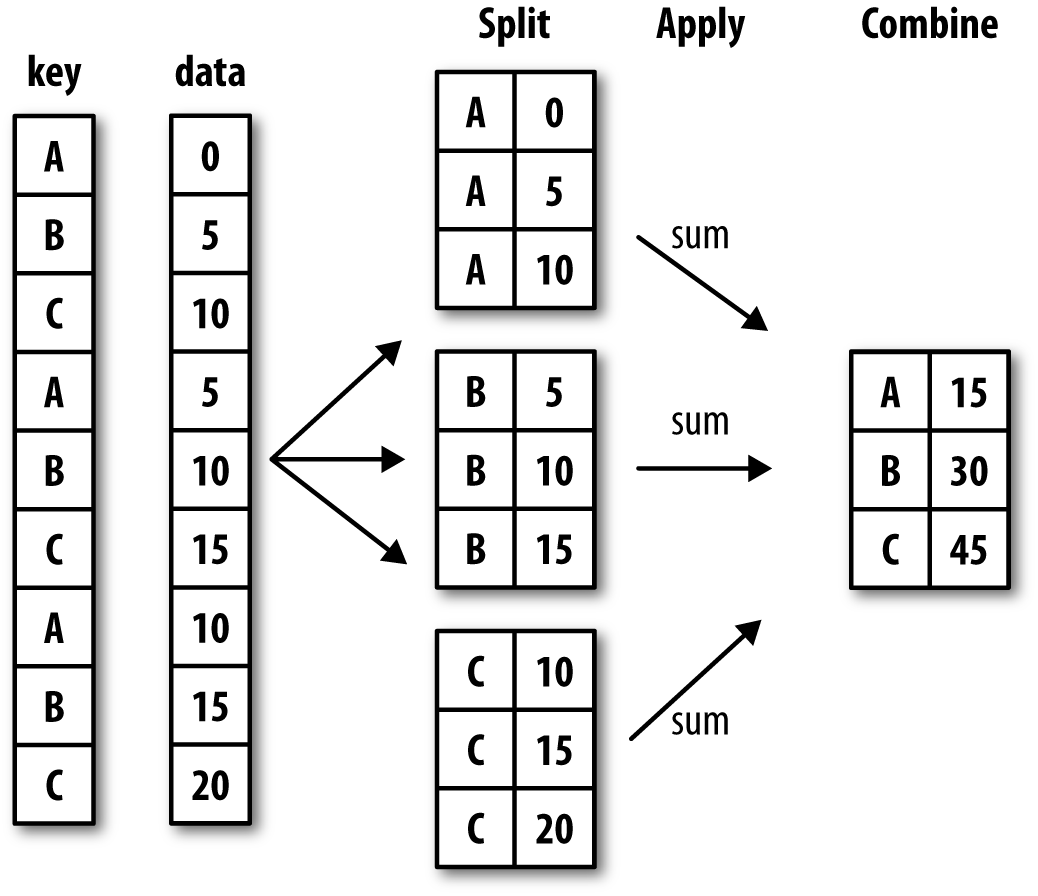
We can do perform this operation using an advanced Pandas method called groupby(), which you can read more about here https://pandas.pydata.org/pandas-docs/stable/user_guide/groupby.html.
GroupBy is popular because it lets you select groups of data and then perform calculations on those smaller groups.
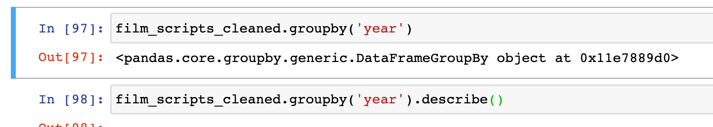
In this example, you’ll notice that we call groupby on the DataFrame and then pass it an argument, in this case the column name year. The column we pass is the one we want to use to aggregate our data. We could also pass in title, but would likely only get groups with one row each.
The output of our groupby() is a new class called DataFrameGroupBy, which is different than a normal DataFrame. Let’s save this to a new variable called films_year, and then try to see what data exists in our group for 2008.
films_year = film_scripts_cleaned.groupby('year')
films_year.get_group(2009)
Running the code should return only the rows that contain the year 2009 in our dataset. Unlike a normal DataFrame, to see the values in a DataFrameGroupBy we need to use the get_group() method, passing it a value from the column we used to aggregate the data.
Or we can perform a calculation on the groupby and turn it back into a normal DataFrame.
Try running this code:
films_year = film_scripts_cleaned.groupby('year')['gross_ia'].sum().reset_index()
Now in a new cell try checking the type() of films_year and print() the value of this variable.
You should see that we now have a DataFrame that contains the total gross for each year. Here’s some other Pandas built-in calculation methods that we could try https://pandas.pydata.org/pandas-docs/stable/user_guide/computation.html#id1
| Pandas method | Explanation |
|---|---|
.count() |
Number of non-NA observations |
.sum() |
Sum of values |
.mean() |
Mean of values |
.median() |
Median of values |
.min() |
Minimum value |
.max() |
Maximum value |
.mode() |
Mode |
.std() |
Sample standard deviation of values |
describe() |
Compute set of summary statistics for Series or each DataFrame column |
You can use these methods on both DataFrame and Series, as well as grouped DataFrame.
You might also take a look at Pandas documentation for using GroupBy https://pandas.pydata.org/pandas-docs/stable/user_guide/groupby.html, especially these diagrams:
Curate and Collect Homework
Now that we’ve learned a bit about Jupyter notebooks and Pandas, your homework assignments is to use both to complete the following assignments. You should create a new folder in your is310-coding-assignments directory called curating-data and then once you have completed the assignments, you should push up your solutions to your repository and link to it in the GitHub discussion for this assignment.https://github.com/ZoeLeBlanc/is310-computing-humanities-2024/discussions/6
Curating The Humanist Dataset Assignment
In class, we worked on getting the text from the Humanist listserv through web scraping. In this assignment, the goal is to complete getting the text from the volumes and to save it to a DataFrame in Pandas. Going forward we’ll be using this dataset to do some initial text analysis.
For this assignment, you should create a Jupyter notebook titled CuratingHumanistData.ipynb and then complete the following tasks:
- Get the text from the Humanist listserv, available here https://humanist.kdl.kcl.ac.uk/Archives/, through web scraping. You can use the code we worked on in class, but you’ll need text from each volume, so be sure to look carefully at the URL structure and how you can use it to get the text from each volume (hint try to look for the link to plain text files). Also make sure you remove all HTML formatting and save the first
10000characters of each volume’s text. - Once your web scraping is working correctly, you will need to decide what other metadata to store with this text data. What information can you get from the
urlvariable? How would you get the years for each volume? (hint checkout thesplit()method in Python). - Finally we have all the data we want to store, so now we have to save it to a Pandas DataFrame and write that DataFrame to
.csvfile calledweb_scraped_humanist_listserv.csv. You can use the following code to save your DataFrame to a.csvfile:
humanist_vols.to_csv('web_scraped_humanist_listserv.csv', index=False)
What does this do to our data? You can read about the to_csv() method here https://pandas.pydata.org/pandas-docs/stable/reference/api/pandas.DataFrame.to_csv.html?highlight=to_csv#pandas.DataFrame.to_csv.
Film Dialogue as Data Advanced Assignment
If you are new to Pandas, this assignment might be a bit too advanced, so just focus on downloading and exploring the data.
For your next assignment, we are returning to The Pudding “Film Dialogue” article https://pudding.cool/2017/03/film-dialogue/ and taking a closer look at some of the data. So far we have worked with the film scripts and now we will bringing in additional data from the The Pudding website.
- Create a new Jupyter notebook called
CuratingFilmDialogue.ipynband read in the three datasets from the Github repository https://github.com/matthewfdaniels/scripts/. Take a look at the documentation in the repository and explore what each file contains, checking if there’s any missing data. - Try to answer the following questions:
- How could we tell if the amount of dialogue was increasing over time in movies? How might this influence the assessment about the breakdown of gender dialogue?
- How could test if there was any relationship between the film’s gross value and the amount of dialogue in the film?
To answer these questions you’ll need to merge, aggregate, and calculate some basic stats for these datasets.
As a bonus, try creating a plot of visualize the answer to each of these questions.
If you get stuck on this assignment, just submit as far as you got and we will discuss it in class.