Advanced Text Analysis

⚡️ This lesson has a notebook with all the code that you can download here. Be sure to download the datasets and correct Python libraries as well.

In the last few classes, we have started to get deeper into text analysis, learning about topics like unsupervised versus supervised modeling, as well as tokenization and vectorization. In this class, we will continue to build on these concepts, learning about more advanced text analysis techniques and how they can help us study cultural data.

From the last class, the assignment was to try and find some patterns in the Humanist Listserv dataset, and specifically to see if we could identify any discourses that were distinctive of the early internet era versus the later web 2.0 era.

To do this, we’re initially going to try out using TF-IDF to see if we can identify any distinctive words or phrases that are associated with these two time periods. We’ll start by loading the Humanist Listserv dataset and then using the TfidfVectorizer from scikit-learn to create a TF-IDF matrix. We’ll then use this matrix to identify the most distinctive words or phrases for each time period.

Here’s the code to do this:

import pandas as pd
import altair as alt
from sklearn.feature_extraction.text import TfidfVectorizer

# Load the Humanist Listserv dataset
humanist_vols = pd.read_csv("web_scraped_humanist_listserv_volumes.csv")

#save our texts to a list
documents = humanist_vols.volume_text.tolist()

#Create a vectorizer
vectorizer = TfidfVectorizer(max_df=.8)
# Fit the vectorizer to our documents
transformed_documents = vectorizer.fit_transform(documents)

# Now get the top features for each document
transformed_documents_as_array = transformed_documents.toarray()

# Get the dates for each volume
dates = humanist_vols.inferred_start_year.tolist()

# Create an empty list to store our results
tfidf_results = []

# Loop through each document and get the top terms
for counter, doc in enumerate(transformed_documents_as_array):
    # Zip together the terms and the scores
    tf_idf_tuples = list(zip(vectorizer.get_feature_names_out(), doc))
    # Sort the terms by score
    one_doc_as_df = pd.DataFrame.from_records(tf_idf_tuples, columns=['term', 'score']).sort_values(by='score', ascending=False).reset_index(drop=True)
    # Add the date to the dataframe
    one_doc_as_df['inferred_start_year'] = dates[counter]
    # Append the dataframe to our list
    tfidf_results.append(one_doc_as_df)
# Concatenate all the dataframes together
tfidf_df = pd.concat(tfidf_results)
# Sort the dataframe by score
tfidf_df = tfidf_df.sort_values(by=['score'], ascending=False)
# Get the top ten terms for each year
top_terms = tfidf_df.groupby('inferred_start_year').apply(lambda x: x.sort_values('score', ascending=False).head(10)).reset_index(drop=True)
# Convert the inferred_start_year to a datetime
top_terms['inferred_start_year'] = pd.to_datetime(top_terms['inferred_start_year'], format='%Y')

Now we should see the following output if we print out the top_terms DataFrame:

	term	score	inferred_start_year
0	num	0.61525	1987-01-01 00:00:00
1	utorepas	0.519124	1987-01-01 00:00:00
2	bitnet	0.232467	1987-01-01 00:00:00
3	vax	0.137863	1987-01-01 00:00:00
4	prolog	0.122248	1987-01-01 00:00:00

This output shows the top ten terms for each year in the Humanist dataset. We can also try visualizing the results using Altair with the following code:

selection = alt.selection_point(fields=['term'], bind='legend')
chart = alt.Chart(top_terms).mark_bar().encode(
    y='score',
    x='inferred_start_year:T',
    color=alt.Color('term', legend=alt.Legend(title='Term', orient='right', symbolLimit=len(top_terms['term'].unique()), columns=5), scale=alt.Scale(scheme='tableau20')),
    tooltip=['term', 'score', 'year(inferred_start_year)'],
    opacity=alt.condition(selection, alt.value(1), alt.value(0.2))
).add_params(selection).properties(
    title='Top 10 Terms by TF-IDF Score in Humanist Volumes'
)
chart

Now clicking on the terms in the legend will highlight the terms in the chart or we can hover over them to see their values. This visualization starts to give us a sense of what terms are most distinctive for each year in the Humanist dataset. Many of these terms are either numbers like years, which would appear uniquely in each volume, or specific terms like “utorepas” or “bitnet” that might be associated with the early internet era. We can also see the rise of digital humanities in the later volumes.

To get at what is most distinctive about the early internet era versus the later web 2.0 era, we can try altering our corpus to group volumes by period and then compare the top terms for each period. We can then use the TfidfVectorizer to create a TF-IDF matrix for each period and compare the top terms for each period. Here’s the code to do this:

# Group the volumes by period
humanist_vols['period'] = pd.cut(humanist_vols['inferred_start_year'], bins=[float('-inf'), 2000, 2010, 2020], labels=['early_internet', 'web_2.0', 'contemporary'])
# Create a vectorizer
vectorizer = TfidfVectorizer(max_df=.8)
# Fit the vectorizer to our documents
transformed_documents = vectorizer.fit_transform(humanist_vols.groupby('period')['volume_text'].apply(' '.join).tolist())
# Now get the top features for each document
transformed_documents_as_array = transformed_documents.toarray()
# Get the periods for each volume
periods = humanist_vols['period'].unique()
# Create an empty list to store our results
tfidf_results = []
# Loop through each document and get the top terms
for counter, doc in enumerate(transformed_documents_as_array):
    # Zip together the terms and the scores
    tf_idf_tuples = list(zip(vectorizer.get_feature_names_out(), doc))
    # Sort the terms by score
    one_doc_as_df = pd.DataFrame.from_records(tf_idf_tuples, columns=['term', 'score']).sort_values(by='score', ascending=False).reset_index(drop=True)
    # Add the date to the dataframe
    one_doc_as_df['period'] = periods[counter]
    # Append the dataframe to our list
    tfidf_results.append(one_doc_as_df)
# Concatenate all the dataframes together
tfidf_df = pd.concat(tfidf_results)
# Sort the dataframe by score
tfidf_df = tfidf_df.sort_values(by=['score'], ascending=False)
# Get the top thirty terms for each period
top_terms = tfidf_df.groupby('period').apply(lambda x: x.sort_values('score', ascending=False).head(30)).reset_index(drop=True)

Now we can visualize the top terms for each period using Altair with the following code:

top_terms['period'] = top_terms['period'].astype(str)
selection = alt.selection_point(fields=['term'], bind='legend')
chart = alt.Chart(top_terms).mark_bar().encode(
    y='score',
    x=alt.X('period', sort=['early_internet', 'web_2.0', 'contemporary'], axis=alt.Axis(title='Period')),
    color=alt.Color('term', legend=alt.Legend(title='Term', orient='right', symbolLimit=len(top_terms['term'].unique()), columns=5), scale=alt.Scale(scheme='tableau20')),
    tooltip=['term', 'score', 'period'],
    opacity=alt.condition(selection, alt.value(1), alt.value(0.2))
).add_params(selection).properties(
    title='Top 30 Terms by TF-IDF Score in Humanist Volumes by Period'
)
chart

So now we are seeing which terms are most distinctive for most period, and we could start researching each term to discover if it is associated with particular technologies or discourses. We could also start to experiment with the hyper-parameters of the TfidfVectorizer to see if we can get more meaningful results.

Hyper-parameters are the settings that we can adjust when we create a model or algorithm. For example, in the TfidfVectorizer, we can adjust the max_df parameter to set the maximum document frequency for a term to be included in the TF-IDF matrix. We could also adjust the min_df parameter to set the minimum document frequency for a term to be included in the TF-IDF matrix. We could also adjust the ngram_range parameter to set the range of n-grams to include in the TF-IDF matrix. By adjusting these hyper-parameters, we can get different results from our TF-IDF analysis.

Unsupervised and Supervised Text Analysis

So far, we have been looking at how to identify distinctive terms in a corpus of text data using TF-IDF, and while this is a powerful algorithm, it is only the tip of the iceberg when it comes to how we can explore textual data. For example, we haven’t really been exploring what words might appear with words related to technology or the internet, or how different words might cluster together in the corpus. To do this we can use something often called clustering to group similar documents together based on the words they contain.

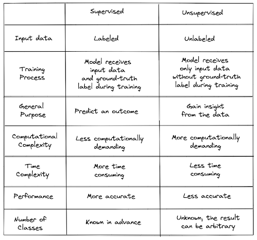
Clustering is an unsupervised machine learning technique that groups similar data points together based on their features. In class we discussed the difference between unsupervised and supervised machine learning, but as a refresher in unsupervised machine learning, we don’t have labeled data, so we are trying to find patterns in the data without knowing what the patterns are. In supervised machine learning, we have labeled data, so we are trying to predict the labels based on the features of the data.

This table gives a good overview of the differences between unsupervised and supervised machine learning:

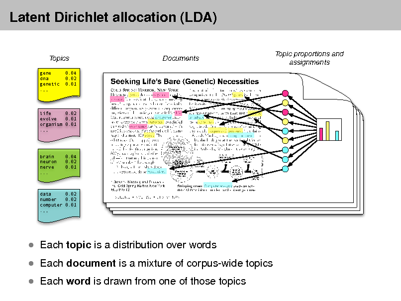
And this figure helps visualize how they work:

Both approaches have their tradeoffs and can be useful in different contexts. For example, unsupervised machine learning can be useful when we don’t have labeled data or when we want to explore patterns in the data without knowing what the patterns are. Supervised machine learning can be useful when we have labeled data and want to predict the labels based on the features of the data. In the case of our Humanist listserv dataset, we don’t have labeled data, so we might want to use unsupervised machine learning to explore patterns in the data.

Topic Modeling

While there are a number of clustering algorithms that we could use to group similar documents together, one of the most popular unsupervised machine learning techniques for text data is topic modeling. Topic modeling is a type of unsupervised machine learning that identifies topics in a corpus of text data. Topic modeling works by identifying groups of words that frequently appear together in the corpus and assigning them to topics. Each topic is a group of words that are related to each other, and each document in the corpus is assigned a distribution over the topics.

We can use scikit-learn and the LatentDirichletAllocation class to perform topic modeling on our Humanist listserv dataset. Here’s the code to do this:

from sklearn.feature_extraction.text import TfidfVectorizer
from sklearn.decomposition import LatentDirichletAllocation
import numpy as np
# Preprocess the text
vectorizer = TfidfVectorizer(max_df=0.8)
tfidf = vectorizer.fit_transform(humanist_vols['volume_text'])

# Perform topic modeling
lda = LatentDirichletAllocation(n_components=len(humanist_vols), max_iter=20, random_state=0)
lda.fit(tfidf)

# Get the top words for each topic
top_words = vectorizer.get_feature_names_out()
topic_words = {}
for topic, comp in enumerate(lda.components_):
    word_idx = np.argsort(comp)[::-1][:10]
    topic_words[topic] = [top_words[i] for i in word_idx]

# Print the top words for each topic
for topic, words in topic_words.items():
    print(f"Topic #{topic}: {', '.join(words)}")

This should give us the following output:

topic	0	1	2	3	4	5	6	7	8	9
0	astra	na	pali	wesolowski	oikawa	hurd	voorhis	texpert	makrolog	ps2
1	xxx	ruhc	kis	hums	riao97	riao	tiiap	bellagio	wipo	nea
2	žikovský	chaffee	chainâ	chainsaw	chaining	chaines	chained	chainbi_at_lycos	chainbi	chaim
3	2003	2002	tocs	0558	mivu	digicult	oesi	m0	eprints	odell
4	epas	aaisp	ceth	etext	8080	netscape	fuer	dsu	hull	908
5	2008	barracuda	esmtp	2002	nz	outbound	messagelabs	helo	ccreegan	asg
6	2014	dhsi	crowdsourcing	dhoxss	cerch	dã	computationalists	ahrc	attachments	fishwick
7	e9	e5	f4	ef	3db7	frankel	e1	3d3d	f0	mw99
8	2004	qs	neach	uottawa	jodi	artfl	tambovtsev	unicode	rs	pmc
9	num	deleted	ninch	htm	cest	wlm	xml	2784	amico	website
10	žikovský	chaffee	chainâ	chainsaw	chaining	chaines	chained	chainbi_at_lycos	chainbi	chaim
11	žikovský	chaffee	chainâ	chainsaw	chaining	chaines	chained	chainbi_at_lycos	chainbi	chaim
12	žikovský	chaffee	chainâ	chainsaw	chaining	chaines	chained	chainbi_at_lycos	chainbi	chaim
13	2014	spf	lemme	helo	forks	dah	pacling	vspace	neder	centerline
14	2016	matlit	livingstone	fã¼r	worldcis	uned	dsh	hcomp	linhd	2017
15	žikovský	chaffee	chainâ	chainsaw	chaining	chaines	chained	chainbi_at_lycos	chainbi	chaim
16	2017	upei	derivational	tandfonline	derimo2017	2018	aclc	hiatt	yisr20	loi
17	žikovský	chaffee	chainâ	chainsaw	chaining	chaines	chained	chainbi_at_lycos	chainbi	chaim
18	2006	ubiquity	fqs	1007	doi	mccarty_at_kcl	2980	3dx	arundel	google
19	digitalhumanities	onlinehome	s16382816	joyent	archiver	postfix	woodward	bounces	dhhumanist	php
20	žikovský	chaffee	chainâ	chainsaw	chaining	chaines	chained	chainbi_at_lycos	chainbi	chaim
21	num	bitnet	utorepas	vax	cst	tlg	kraft	cdt	wordperfect	ccat
22	žikovský	chaffee	chainâ	chainsaw	chaining	chaines	chained	chainbi_at_lycos	chainbi	chaim
23	2007	2008	wmccarty	fludd	infinitum	1617	ahrc	jiia	tl	ichim07
24	žikovský	chaffee	chainâ	chainsaw	chaining	chaines	chained	chainbi_at_lycos	chainbi	chaim
25	žikovský	chaffee	chainâ	chainsaw	chaining	chaines	chained	chainbi_at_lycos	chainbi	chaim
26	2011	a0	fractional	interedition	pocos	mw2012	kflc	jascha	utpjournals	dh2012
27	žikovský	chaffee	chainâ	chainsaw	chaining	chaines	chained	chainbi_at_lycos	chainbi	chaim
28	žikovský	chaffee	chainâ	chainsaw	chaining	chaines	chained	chainbi_at_lycos	chainbi	chaim
29	2018	mailing_list_multi	fish	benzon	lâ	fatal	mathophobia	flaws	yisr20	dâ
30	1998	ftp	gopher	marchand	cti	5801	ippe	tact	___	brians
31	žikovský	chaffee	chainâ	chainsaw	chaining	chaines	chained	chainbi_at_lycos	chainbi	chaim
32	cultivate	ucita	gratias	agere	dchamber	evtoc	primitives	www10	evelyn	virilio

You’ll notice that I’m setting the number of topics to be the same as the number of volumes in the Humanist dataset. This is because the LatentDirichletAllocation algorithm requires us to specify the number of topics, and in this case, we are trying to identify topics for each volume in the dataset. We could also try setting the number of topics to a smaller number to see if we can identify broader topics in the dataset or change our TF-IDF parameters to see if that leads to more distinctive words being surfaced.

Classifiers

Alternatively, we could use supervised machine learning techniques to predict the time period of each volume in the Humanist dataset based on the words they contain. This would involve training a classifier on a subset of the data where we know the time period of each volume and then using the classifier to predict the time period of the remaining volumes. This is a common approach in text analysis when we have labeled data and want to predict the labels based on the features of the data.

In our case, we might want to use our earlier periods as labels and then try to predict which terms are most distinctive of each period. We could then use these terms to predict the time period of the remaining volumes in the dataset. Here’s the code to do this:

from sklearn.model_selection import train_test_split
from sklearn.feature_extraction.text import TfidfVectorizer
from sklearn.linear_model import LogisticRegression
from sklearn.metrics import classification_report

# Create a vectorizer
vectorizer = TfidfVectorizer(max_df=0.8)
# Fit the vectorizer to our documents
transformed_documents = vectorizer.fit_transform(humanist_vols['volume_text'])

# Split the data into training and test sets
X_train, X_test, y_train, y_test = train_test_split(transformed_documents, humanist_vols['period'], test_size=0.2, random_state=0)

# Train a logistic regression classifier
clf = LogisticRegression(max_iter=1000)
clf.fit(X_train, y_train)

# Predict the time period of the test set
y_pred = clf.predict(X_test)

# Print the classification report
print(classification_report(y_test, y_pred))

Which gives us the following results:

	precision	recall	f1-score	support
contemporary	1	0.333333	0.5	3
early_internet	1	1	1	2
web_2.0	0.5	1	0.666667	2
accuracy	0.714286	0.714286	0.714286	0.714286
macro avg	0.833333	0.777778	0.722222	7
weighted avg	0.857143	0.714286	0.690476	7

This is telling us how well our classifier is doing at predicting the time period of each volume in the Humanist dataset. We can see that the classifier is doing pretty well, with an accuracy of 0.71, which means that it is correctly predicting the time period of each volume about 71% of the time. You’ll notice that it is doing better at predicting the early internet and web 2.0 periods than the contemporary period, which might be because the contemporary period is more similar to the web 2.0 period than the early internet period.

We could also extract the terms most associated with each period using the following code:

# Get the coefficients for each term
coefficients = clf.coef_
# Get the terms
terms = vectorizer.get_feature_names_out()
# Create a dataframe of the terms and coefficients
terms_df = pd.DataFrame({'term': terms, 'contemporary': coefficients[0], 'early_internet': coefficients[1], 'web_2.0': coefficients[2]})
# Get the top terms for each period
top_terms = terms_df.melt(id_vars='term', var_name='period', value_name='coefficient').sort_values(by='coefficient', ascending=False).groupby('period').head(10)

This gives us the following output:

term	period	coefficient
num	early_internet	1.21206
digitalhumanities	contemporary	1.01717
2006	web_2.0	0.480645
onlinehome	contemporary	0.474791
s16382816	contemporary	0.474791
2002	web_2.0	0.456101
joyent	web_2.0	0.356053
bitnet	early_internet	0.341151
2008	web_2.0	0.307246
dhhumanist	contemporary	0.296768
archiver	contemporary	0.285431
cest	contemporary	0.270183
2003	web_2.0	0.250799
woodward	web_2.0	0.244343
2007	web_2.0	0.241049
esmtp	web_2.0	0.220966
2009	web_2.0	0.209739
barracuda	web_2.0	0.196746
2015	contemporary	0.195885
deleted	early_internet	0.192321
postfix	contemporary	0.191936
ninch	web_2.0	0.180353
ubiquity	web_2.0	0.175565
ftp	early_internet	0.174169
1007	web_2.0	0.170139
2016	contemporary	0.165034
doi	web_2.0	0.161822
2017	contemporary	0.149745
utorepas	early_internet	0.147523
2014	contemporary	0.133621
gopher	early_internet	0.130811
listmember_interface	contemporary	0.124616
htm	web_2.0	0.123987
php	contemporary	0.123323
fqs	web_2.0	0.120207
ppp	contemporary	0.119089
vax	early_internet	0.119023
spam	contemporary	0.113921
3dx	web_2.0	0.110824
mccarty_at_kcl	web_2.0	0.110779
autolearn	contemporary	0.108205
all_trusted	contemporary	0.108185
10009	contemporary	0.108185
epas	early_internet	0.106211
nz	web_2.0	0.105384
bayes_00	contemporary	0.105316
arundel	web_2.0	0.103139
xml	web_2.0	0.0991835
spamassassin	contemporary	0.0983372
bounces	contemporary	0.0963914
7848	web_2.0	0.0939354
userid	contemporary	0.0937591
infobits	web_2.0	0.0908213
messagelabs	web_2.0	0.0893617
aaisp	web_2.0	0.0881107
outbound	web_2.0	0.0877741
2013	contemporary	0.0827581
vhost	contemporary	0.0808539
wlm	web_2.0	0.079479
wikipedia	web_2.0	0.0789063
asg	web_2.0	0.0786985
tlg	early_internet	0.0785648
qs	early_internet	0.0773452
2784	web_2.0	0.0771147
cst	early_internet	0.0748274
uribl_blocked	contemporary	0.0744614
ichim99	early_internet	0.0687415
kraft	early_internet	0.0599564
beenthere	contemporary	0.0591908
membership_form	contemporary	0.0587342
listmember	contemporary	0.0564102
ham	contemporary	0.0561662
cdt	early_internet	0.0557935
ccat	early_internet	0.0549989
spf	contemporary	0.0546195
ippe	early_internet	0.0529816
pst	early_internet	0.0520612
wordperfect	early_internet	0.0517592
cti	early_internet	0.0487855
marchand	early_internet	0.0480226
coombs	early_internet	0.0474053
xxx	early_internet	0.0466514
brownvm	early_internet	0.0463937
cni	early_internet	0.04483
ceth	early_internet	0.0447585
bene	early_internet	0.0445725
brians	early_internet	0.0445527
osher	early_internet	0.044098
neach	early_internet	0.0438512
wordcruncher	early_internet	0.0428789

We can then visualize the top terms for each period using Altair with the following code:

# visualize top terms
top_terms['period'] = top_terms['period'].astype(str)
selection = alt.selection_point(fields=['term'], bind='legend')

# Define the sort order for the periods
period_order = ['early_internet', 'web_2.0', 'contemporary']

chart = alt.Chart(top_terms).mark_bar().encode(
    x=alt.X('period', sort=['early_internet', 'web_2.0', 'contemporary'], axis=alt.Axis(title='Period')),
    y=alt.Y('coefficient:Q'),  # Sort terms by score in descending order
    color=alt.Color('term', legend=alt.Legend(title='Term', orient='right', symbolLimit=len(top_terms['term'].unique()), columns=5), scale=alt.Scale(scheme='tableau20')),
    tooltip=['term', 'coefficient', 'period'],
    opacity=alt.condition(selection, alt.value(1), alt.value(0.2))
).add_params(selection).properties(
    title='Top 10 Terms by Coefficient in Logistic Regression Model by Period'
)
chart

Now we have officially experimented with two types of machine learning!! We could also try other classifiers like RandomForestClassifier or SVM to see if we get different results. We could also try different hyper-parameters for the TfidfVectorizer to see if we get different results. We could also try different feature selection techniques to see if we get different results. There are many ways to experiment with text analysis, and the more you experiment, the more you’ll learn about the data and the algorithms.

Resources

We have only briefly touched on the possibilities of text analysis in this lesson. There are many more techniques and algorithms that you can use to explore textual data. Here are some resources to help you learn more about text analysis:

• Thomas Jurczyk, “Clustering with Scikit-Learn in Python,” Programming Historian 10 (2021), https://doi.org/10.46430/phen0094.
• Matthew J. Lavin, “Regression Analysis with Scikit-Learn (part 1 - Linear),” Programming Historian 11 (2022), https://doi.org/10.46430/phen0099.
• Matthew J. Lavin, “Regression Analysis with Scikit-Learn (part 2 - Logistic),” Programming Historian 11 (2022), https://doi.org/10.46430/phen0100.
• John R. Ladd, “Understanding and Using Common Similarity Measures for Text Analysis,” Programming Historian 9 (2020), https://doi.org/10.46430/phen0089.
• Matthew J. Lavin, “Analyzing Documents with TF-IDF,” Programming Historian 8 (2019), https://doi.org/10.46430/phen0082.