Introduction to Cleaning and Working With Data

⚡️ This lesson has been adapted from Heather Froehlich's A Gentle Introduction To Excel And Spreadsheets For Humanities People https://hfroehli.ch/2021/06/17/a-gentle-introduction-to-excel-and-spreadsheets-for-humanities-people/

So far we have been talking about file formats and trying our hand at creating data, but what about best practices for this work? And what does it mean to work with data in the humanities?

What is Humanities Data and How Can We Work with It?

As you’ve read this week, there’s no one definition of or way to work with humanities data, especially since the very category of ‘humanities’ itself is contested and nebulous. One of the key things that you’ve hopefully learned from our assignment this week is that creating data is a process that requires many interpretative steps and that it can difficult to know how to proceed if you don’t have a clear goal in mind.

As Posner writes:

“It requires some real soul-searching about what we think data actually is and its relationship to reality itself; where is it completely inadequate, and what about the world can be broken into pieces and turned into structured data? I think that’s why digital humanities is so challenging and fun, because you’re always holding in your head this tension between the power of computation and the inadequacy of data to truly represent reality.”

While hopefully we have discussed some of the choices everyone made in their dataset creation assignment, I also wanted to share my attempt at creating this dataset.

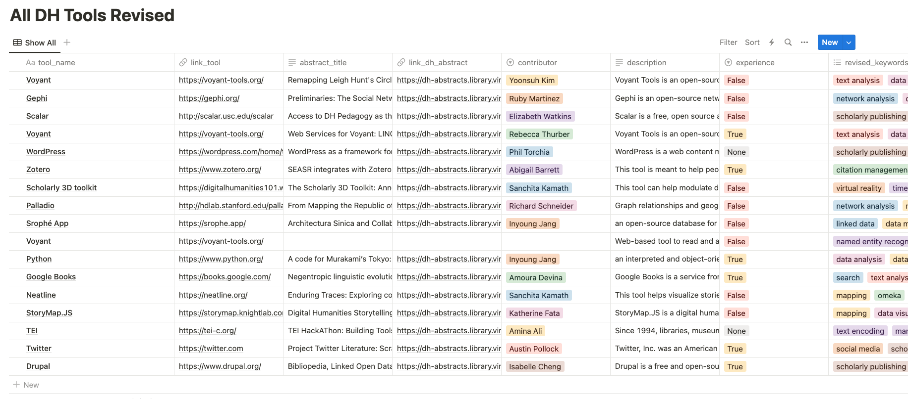Click on the image to see my dataset

As I mentioned in class, when manually cleaning data, I often use Notion (though you can do this work in Google Sheets, Excel, AirTable, etc…). In my example, you can see I’ve made a few interpretative choices from our original dataset from class:

1. I have renamed all the column names to be lowercase and underscored. This is a common practice in datasets since it is easier for computers to autocomplete and requires less typing, depending on the software you are using.
2. I have changed the description column to contains True, False, None which are values that work better with computers rather than Yes or No.
3. I have filled in as many of the missing values as I could. But I also created a column called abstract_original so that I could keep track of whether a contributor had initially submitted an abstract or if it was one I found. This choice was so that I was not skewing the initial records but still had a way to fill in missing values.
4. I also created a column called revised_keywords where I combined our two categorical columns (Tool Category and Area of Use) and also limited the number of values. This choice is very subjective and I could have made different choices, but I wanted to limit the number of values to make it easier to work with the data. The more options you have, the more complexity you create.
5. Lastly, I used some of the built-in Notion functionality to color some of the values. This makes it easier for me to look at the data, but it is important to note that computers do not understand colors. So if I wanted to use this data in a visualization, I would need to create a new column that would translate the colors into values that computers can understand.

All of these choices are subjective and represent my own interpretation of the data. But they are also choices that I made to make it easier to work with the data down the road. One of the reasons I use Notion is also because this lets me export the data as a Markdown File and CSV, which you can also find in the GitHub repository.

Dataset Foundations

From this experience of creating data, you are starting to learn that creating datasets requires taking unstructured data and giving it some type of structured format. In other fields, you will often be given data from the outset that is already created but in DH, a lot of the work requires making your own data and thinking about how it should be organized.

A great example of this is the Shakespeare and Company Project at Princeton which has digitized lending library cards to build their project:

You can read more about the project here https://shakespeareandco.princeton.edu, but there are some key principles that will help you as you continue to do this work, even if the software you use will differ.

1. Datasets are made up of rows and columns. Each row represents a single record and each column represents a single variable. So for example, a row might be a single book and the columns might be the title, author, and publication date. Or in our case a row might be a single DH tool and the columns might be the name, description, and category.
2. Single values are often called cells. These cells are the intersection of a row and column, and can contain many types of data. Often a rule of thumb is that a cell should contain a single observation or data point, but this is a general rule and not always the case.
3. The first row of a dataset is often called the header row. This row contains the column names and is often used to describe the data in the dataset. Naming columns is an important part of creating a dataset because it helps you and others understand what the data represents.
4. Many spreadsheet software allow you to have multiple sheets (like Google Sheets for example), or you might try to add multiple datasets on one sheet like we did in class last week. Another general rule of thumb is that each sheet should contain a single dataset. This is because it makes it easier to work with the data and to share it with others.
5. Finally, it is important to remember that this is not a text document so it is crucial to work with these softwares in ways the expect. For example, many of these softwares might try to automatically deduce your data from the formatting, so if you have dates you might want to structure it as YYYY-MM-DD or if you have numbers you might want to remove any commas or dollar signs. This is because computers do not understand the same things as humans, so we need to make sure that we are structuring our data in a way that computers can understand.

Here’s an example from Google Sheets:

And you can read more about these foundations here: https://sheetshelp.com/spreadsheet-parts/

Data Types

Now let’s trying working in Google Sheets again with this revised All DH Tools dataset to start understanding some of the foundations of working with data.

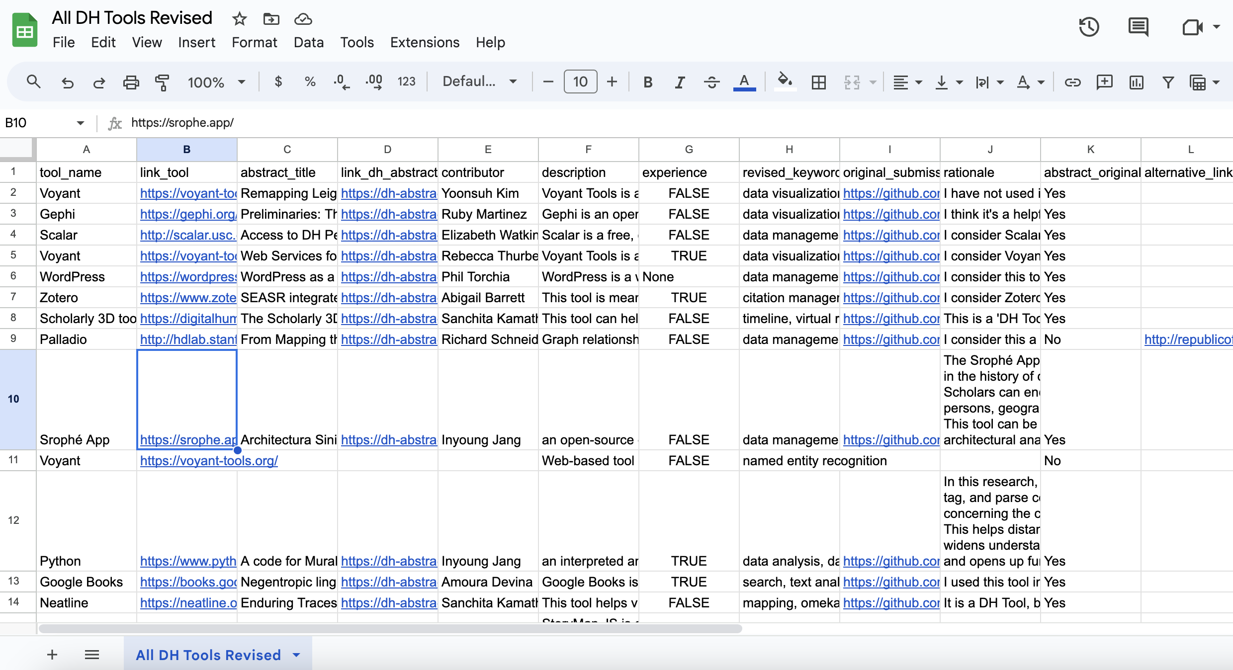
Here’s an uploaded version of the dataset I created in Notion. You’ll notice a few things immediately. First, all the colors are gone as predicted. You’ll also see that all the links are automatically rendering as links, and that experience is also rendering as TRUE and FALSE versus abstract_original which was a checkbox in Notion that is now rendered as Yes or No since that was how Notion exported that format.

When working with data it is crucial to understand that there are different types of data.

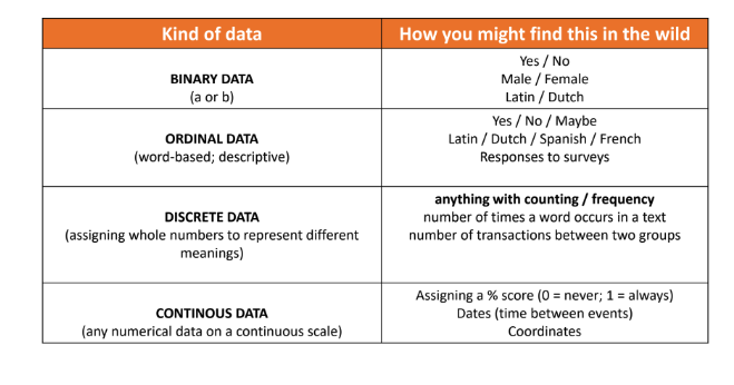
Using this graph we can see that our data is primarily categorical from tool_name to description, etc… But we also have some boolean data in experience and abstract_original. Boolean is a fancy way of saying True or False. We also have a None value in abstract_original which is a way of saying that there is no value in that cell. Explicitly stating that there is no value can be useful so that there’s no ambiguity, though most spreadsheet software will automatically assume empty cells contain None (which is also called a Null value).

You will also see that my revised_keywords column now has commas to separate our keywords. When working with a list of items in a cell, it is good practice to use some type of symbol that can be a delimiter. Most software assumes that commas or semi-colons are delimiters, and by having this standard format it will allow you to more easily work with this data.

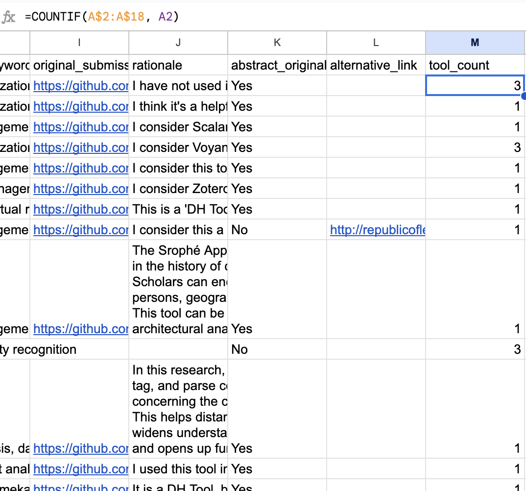
We can try creating some derived numerical data from our current dataset through Google Sheets. Derived data is a termed often used to denote any aggregation or transformation of a dataset to create additional data that was not there originally.

One thing we might want to know is how popular these tools are across the class. We can get some help through ChatGPT to find the exact syntax, through using the following prompt:

I have a Google Sheets dataset with the following columns: tool_name, link_tool, abstract_title, link_dh_abstract, contributor, description, experience, revised_keywords, original_submission, rationale, abstract_original, alternative_link. I want to know how many times each tool was used and save that into a new column called tool_count. tool_name is in column A and I want tool_count to be in column M. There is also 18 rows including the header column. My sheet is also called All DH Tools Revised. How can I do this?

And from ChatGPT we learn that:

Given your dataset and the specified columns, here’s how you can determine how many times each tool was used and save that into the tool_count column:

1. Column Headers: Assuming you have your headers in row 1, type “tool_count” in cell M1 to label the new column.

2. Count Formula: In cell M2, right next to the first tool name in column A, you will use the COUNTIF function to calculate the number of times that tool appears in the tool_name column.

   Enter the following formula in cell M2:

   =COUNTIF(A$2:A$18, A2)
   

3. Drag Down the Formula: After entering the formula in cell M2, you can click on the bottom-right corner of the cell (where there’s a little square or “handle”) and drag it down to fill cells M2 through M18. This will apply the formula to each row, counting occurrences of the corresponding tool in column A.

4. Result: Now, column M will contain the count of each tool listed in column A for all rows 2 through 18.

Remember, the absolute reference ($ in A$2:A$18) ensures that as you drag the formula down, it will always count against the entire specified range, whereas the relative reference (A2) updates for each row you drag to.

If done correctly, we should get a result that looks like this:

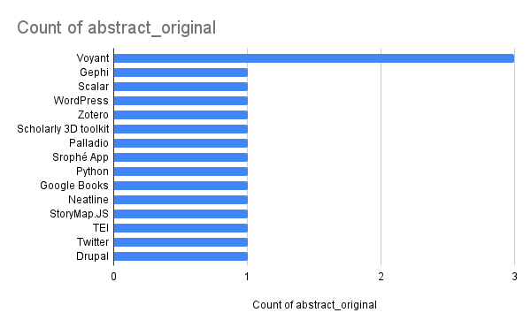
We can also visually examine the popularity of tools by creating a bar chart. Using the graph button in Google Sheets to see the most popular tools:

Data Merging and Filtering

Now that we have our own dataset, let’s try and work with some other datasets to compare our results.

First, we can have the data from Barbot, Laure, Frank Fischer, Yoann Moranville, and Ivan Pozdniakov. “Which DH Tools Are Actually Used in Research?,” December 6, 2019. https://weltliteratur.net/dh-tools-used-in-research/, which should download as tools-dh-proceedings.csv. Let’s open this up in Google Sheets and try and connect it to our existing dataset to compare the popularity of these tools.

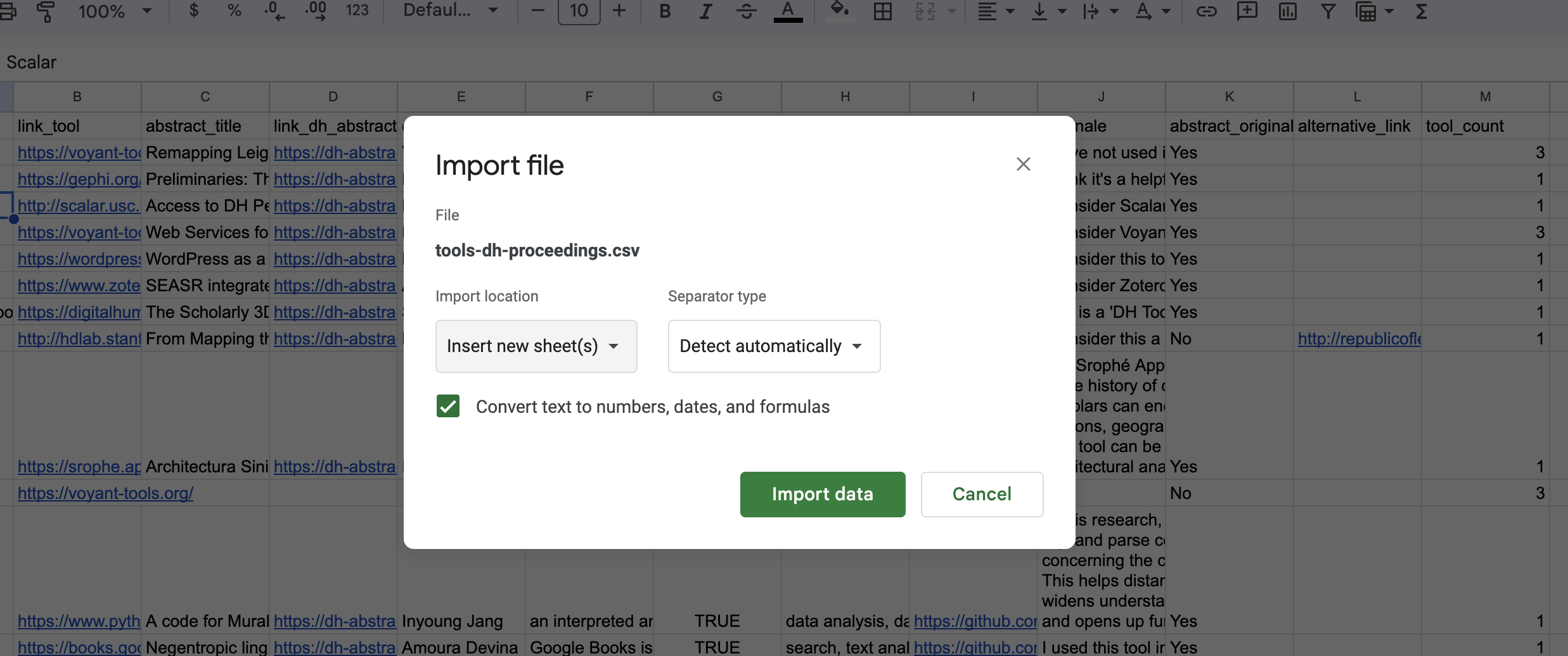
First, we need to import this data into our existing spreadsheet but as a separate sheet. Under File we can select the import option and then upload our csv file.

Now we should have a sheet called tools-dh-proceedings at the bottom of our spreadsheet. Next we can once again ask ChatGPT for help by using the following prompt:

I have a Google Sheets dataset with two sheets. The first is called All DH Tools Revised with the following columns: tool_name, link_tool, abstract_title, link_dh_abstract, contributor, description, experience, revised_keywords, original_submission, rationale, abstract_original, alternative_link, tool_count. The second is called tools-dh-proceedings with the following columns: Tool, 2015, 2016, 2017, 2018, 2019. How can I merge these two datasets into a single dataset? The Tool column contains the same information but there are fewer rows in the first dataset than the second. Should I rename the two columns to match?

And we get this answer from ChatGPT:

Yes, renaming the header “Tool” to “tool_name” in the tools-dh-proceedings sheet would simplify the merging process a bit, especially when viewing or referencing the data. If you do that, here’s a more streamlined approach:

1. Create a New Sheet:
   • Add a new sheet by clicking the “+” button at the bottom-left of the Google Sheets interface. Name it something like “Merged Dataset”.
2. Copy the Headers:
   • Copy the headers from the All DH Tools Revised sheet and paste them into the new “Merged Dataset” sheet.
   • After the last column from All DH Tools Revised, copy the headers from 2015 to 2019 in the tools-dh-proceedings sheet and paste them next to the previously pasted headers in “Merged Dataset”.
3. Transfer the Data from All DH Tools Revised:
   • Copy all the data from the All DH Tools Revised sheet (excluding the header row) and paste it into the “Merged Dataset” sheet below the corresponding headers.
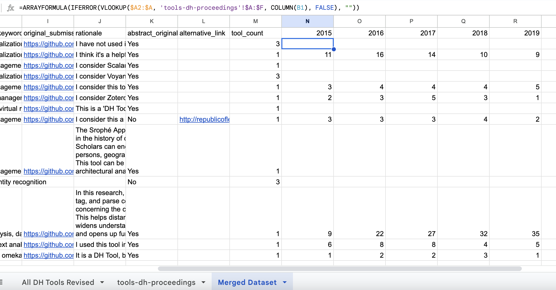
4. Use ARRAYFORMULA with VLOOKUP for the Remaining Columns:
   • Assuming the data from All DH Tools Revised starts in row 2 of the “Merged Dataset” sheet, in the next available column (which corresponds to 2015), input the following formula in the cell corresponding to row 2:

     =ARRAYFORMULA(IFERROR(VLOOKUP($A2:$A, 'tools-dh-proceedings'!$A:$F, COLUMN(B1), FALSE), ""))
     

   • Drag this formula to the right for the years 2016, 2017, 2018, and 2019. Adjust the COLUMN(B1) part to COLUMN(C1), COLUMN(D1), etc., respectively, as you move right.

5. Explanation: The VLOOKUP function searches for each tool name from the “Merged Dataset” sheet in the tool_name column of the tools-dh-proceedings sheet. The ARRAYFORMULA allows the VLOOKUP to process multiple rows at once. If a match is found, it fetches the corresponding year’s data. If not, it returns an empty string (due to the IFERROR function).

6. Tidy Up: After merging, verify the data to check for any discrepancies or errors. If you wish, you can replace formulas with static values (by copying the columns and using “Paste Special” > “Paste Values Only”) to prevent accidental recalculations or errors if the original data is modified.

Now you should have a more easily managed merged dataset with the data from both sheets based on the “tool_name” headers.

We can even ask ChatGPT how to alter our formula so that it includes zeros instead of empty cells:

=ARRAYFORMULA(IF(A2:A18="", "", IFERROR(VLOOKUP($A2:$A18, 'tools-dh-proceedings'!$A:$F, COLUMN(B1), FALSE), 0)))

⚡️ I have filmed the remainder of the tutorial and posted the video here since we did not complete everything during class https://mediaspace.illinois.edu/media/t/1_4itob4ov. Please reach out on Slack if you have any questions or difficulty watching the video

VLOOKUP and Google Sheets Documentation

As ChatGPT explains briefly, VLOOKUP is a built-in function that stands for “Vertical Lookup” and exists in most spreadsheet software. It searches for a value in the first column of a table range and returns a corresponding value from another column in the same row. Essentially, VLOOKUP helps in cross-referencing data. The function can be immensely valuable when trying to integrate information from different tables or datasets based on a common identifier.

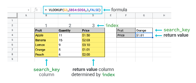
To explain it in a bit more depth, the VLOOKUP function takes four arguments:

1. Search Key: The value to search for in the first column of the table range. In our case, this is the tool name from the “Merged Dataset” sheet.

2. Table Range: The range of cells that contains the data to be searched. In our case, this is the tool_name column from the tools-dh-proceedings sheet.

3. Column Index: The column number of the table range from which to return a value. In our case, this is the column number of the year’s data (e.g., 2015 is column 2, 2016 is column 3, etc.).

4. Is Sorted: A boolean value that indicates whether the first column of the table range is sorted in ascending order. In our case, this is FALSE because the tool_name column is not sorted.

The IFERROR function is used to handle errors that may occur when the VLOOKUP function is unable to find a match. In our case, if a match is not found, the VLOOKUP function returns an error, which is then replaced with an empty string by the IFERROR function.

The ARRAYFORMULA function allows the VLOOKUP function to process multiple rows at once. Without this function, you would have to copy the VLOOKUP formula to each row individually.

The COLUMN function returns the column number of a specified cell reference. In our case, we use COLUMN(B1) to return the column number of the cell in column B (i.e., column 2).

This is a lot of technical information that while helpful to know is not critical to memorize, instead you can find most of this information in the help documentation for your software. For example, here’s the help documentation for Google Sheets: https://support.google.com/docs/answer/3093318?hl=en. Learning to read documentation is a helpful skill so while ChatGPT and other tools can help you get started, it is important to learn how to read documentation and to understand the basics of how your software works.

---

Let’s try and merge these two datasets in a different way to make sure we are fully understanding how to do this. This time lets merge All DH Tools Revised into tools-dh-proceedings using similar steps:

• First, we need to create a new Google Sheet called Reversed Merged Dataset.

• Then we need to once again copy the headers from each sheet, along with the full data from tools-dh-proceedings. Though remember to not repeat tool_name in the Reversed Merged Dataset sheet.

• Next, we can use ChatGPT to help us with the formula to merge the data from All DH Tools Revised into Reversed Merged Dataset:

I have a Google Sheets dataset with two sheets. The first is called tools-dh-proceedings with the following columns: tool_name, 2015, 2016, 2017, 2018, 2019. The second is called All DH Tools Revised with the following columns: tool_name, link_tool, abstract_title, link_dh_abstract, contributor, description, experience, revised_keywords, original_submission, rationale, abstract_original, alternative_link, tool_count. How can I merge these two datasets into a single dataset? In this instance, I want to merge All DH Tools Revised into tools-dh-proceedings. The tool_name column contains the same information but there are fewer rows in the first dataset than the second. tools-dh-proceedings has a range from A1:F239 including the header column and All DH Tools Revised has a range of A1:M18 including the header column. I want to save this merged dataset in a new sheet called Reversed Merged Dataset. Help me write this formula.

ChatGPT gives us the following answer:

1. In cell A2 of your Reversed Merged Dataset sheet, write the following formula to bring over all data from tools-dh-proceedings:

    =ARRAYFORMULA('tools-dh-proceedings'!A2:F239)
   

   Notice that we had previously manually copied the data, but ChatGPT is sharing that we can use ARRAYFORMULA to do this programatically

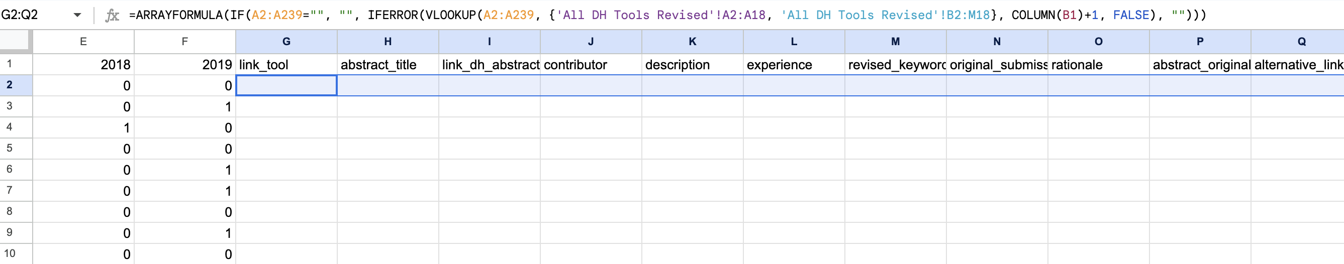
2. In cell G2 of your Reversed Merged Dataset sheet, use the following formula to bring over data from All DH Tools Revised based on the tool_name:

    =ARRAYFORMULA(IF(A2:A239="", "", IFERROR(VLOOKUP(A2:A239, {'All DH Tools Revised'!A2:A18, 'All DH Tools Revised'!B2:M18}, COLUMN(B1)+1, FALSE), "")))
   

   • The IF(A2:A239="", "", ...) part checks if the tool_name is empty and skips the empty rows.
   • VLOOKUP(A2:A239, {'All DH Tools Revised'!A2:A18, 'All DH Tools Revised'!B2:M18}, COLUMN(B1)+1, FALSE) performs a lookup based on tool_name to get corresponding values from the second dataset.
   • The COLUMN(B1)+1 dynamically calculates the column index for the data from All DH Tools Revised so that it starts from column B (link_tool) in that sheet.

3. Drag this formula across from column G to column O so that it fetches all remaining columns from All DH Tools Revised.

While this formula largely works, when we drag it across columns, you’ll notice that it is not autopopulating our data.

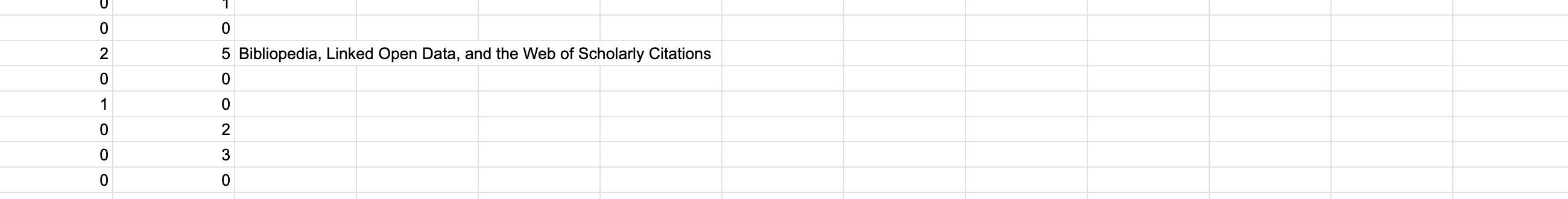
Instead we need to ask ChatGPT to tweak the formula to work with multiple columns (otherwise we would have to update the formula for each column):

=ARRAYFORMULA(
   IF(A2:A239="", "", 
      IFERROR(VLOOKUP(A2:A239, 'All DH Tools Revised'!A2:M18, SEQUENCE(1, 12, 2), FALSE), "")
   )
)

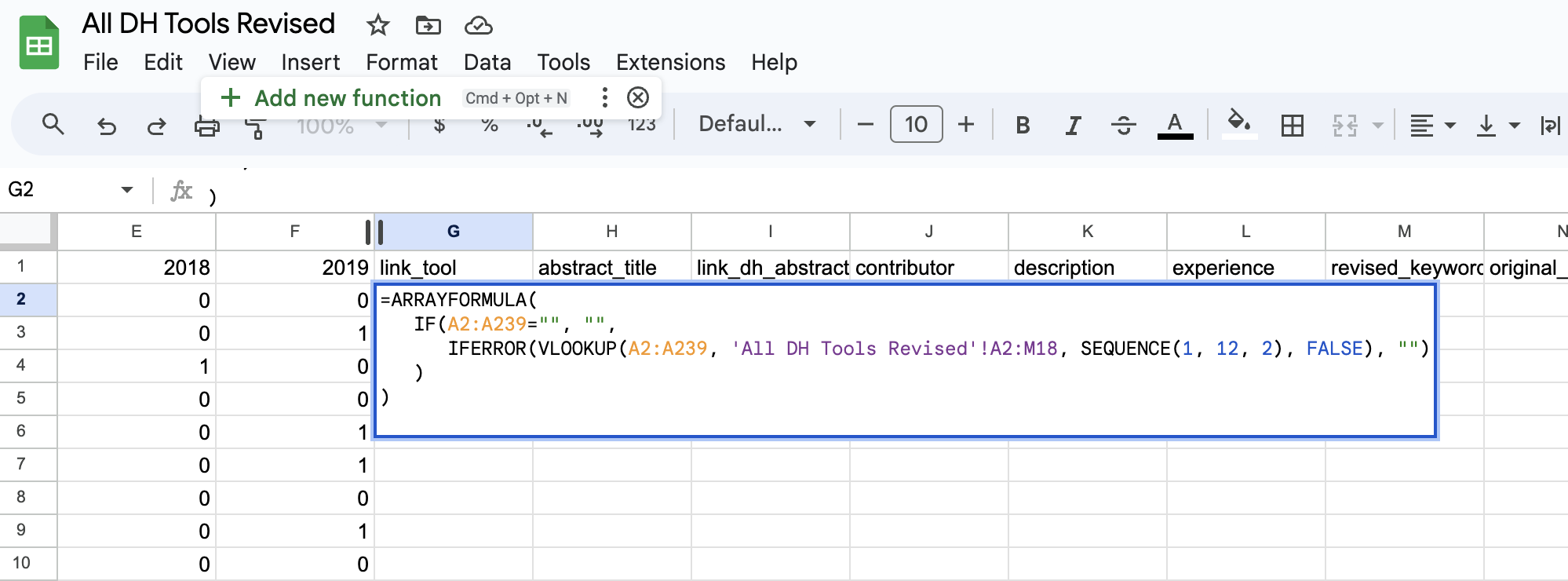
When we enter this revised formula, we’ll see an option to add a new function, which we can do by clicking on the + button (this is optional though).

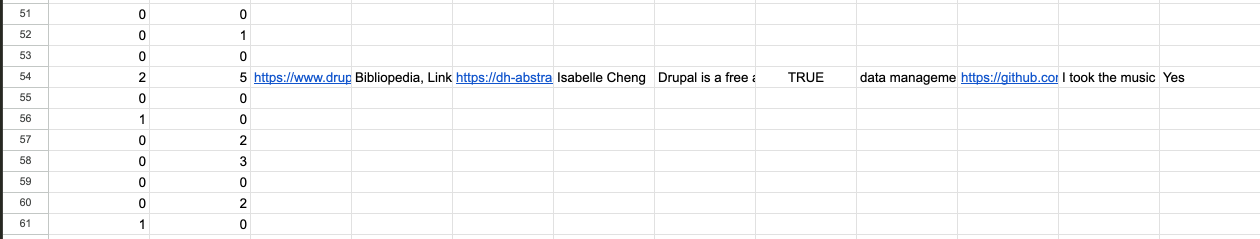
Once we click on the + button, we should see that our data has been merged successfully if we scroll down.

Optional In-Depth Explanation

While we are largely using ChatGPT to help us with this work, it is important to understand what is happening in this formula.

ARRAYFORMULA

=ARRAYFORMULA(...)

This function allows you to perform a calculation or operation over an entire range of cells rather than just a single one. In the context of the formula you provided, it enables the subsequent functions (IF, IFERROR, and VLOOKUP) to operate over arrays of cells rather than just individual ones.

IF

IF(A2:A239="", "", ...)

This is a condition that checks whether the cells from A2 to A239 are empty. The logic is:

• If they’re empty (A2:A239=""), it returns an empty string, essentially ignoring that row.
• If they’re not empty, it proceeds to evaluate the next portion of the formula.

IFERROR

IFERROR(VLOOKUP(...), "")

This function checks if the inner function (VLOOKUP in this case) returns an error. If VLOOKUP results in an error, rather than displaying that error, IFERROR will return an empty string (“”). This is especially useful for tidying up the spreadsheet so that if there’s no match found by VLOOKUP, the cell doesn’t display a distracting error message but instead remains blank.

VLOOKUP

VLOOKUP(A2:A239, 'All DH Tools Revised'!A2:M18, SEQUENCE(1, 12, 2), FALSE)

This is the primary function doing the data fetching and merging:

• A2:A239: This is the lookup range. For each cell value in this range, VLOOKUP will attempt to find a matching value in the first column of the provided table range.

• 'All DH Tools Revised'!A2:M18: This is the table array where VLOOKUP searches for the lookup value. In this case, it’s searching within another sheet titled “All DH Tools Revised” from columns A to M.

• SEQUENCE(1, 12, 2): This is the dynamic column index that tells VLOOKUP which column(s) to return once a match is found.

• SEQUENCE(1, 12, 2) generates a virtual array: [2, 3, 4, … 13]. Here’s the breakdown of its parameters:

  • 1: Number of rows for the sequence (in this case, just one row).
  • 12: Number of columns, so we get 12 sequential numbers.
  • 2: Start value; the sequence starts from 2.

Since VLOOKUP usually returns a single column, combining it with SEQUENCE in an ARRAYFORMULA effectively makes it fetch multiple columns dynamically.

• FALSE: This ensures VLOOKUP looks for an exact match.

Summary

To put it all together: For each non-empty cell in the range A2 to A239, the formula will look up its value in the ‘All DH Tools Revised’ sheet within columns A to M. If it finds a match, it will return the corresponding values from columns B to M (12 columns) of that sheet. If it doesn’t find a match or encounters any other error, it will leave the cell blank.

Cleaning Large Datasets with OpenRefine

So far we have joined our dataset with the tools-dh-proceedings data but we also have the Index of DH Conferences that contains relevant potential data for our dataset. Let’s try and merge these two datasets together.

We can download the simple csv dataset from here https://dh-abstracts.library.virginia.edu/downloads and that should download a zip file that when opened contains a csv file called dh_conferences_works.csv. As we tried in class though, this file is much larger, containing over 8000 rows. So instead we need to use a program called OpenRefine to help us clean this data.

OpenRefine is a popular tool in DH because it is both free and open source, but also because it is a powerful tool for cleaning data. You can download OpenRefine here: https://openrefine.org/download.

Once you have downloaded and installed the tool (remember to reach out if you have issues), you should see the following interface:

You’ll notice that the url bar at the top has a strange series of numbers or might include something like localhost. All that means is that this is a local server running on your computer. You can think of it like a website that is only accessible on your computer. This is important to know because it means that you can only access this data on your computer, so if you want to share it with others you will need to export it.

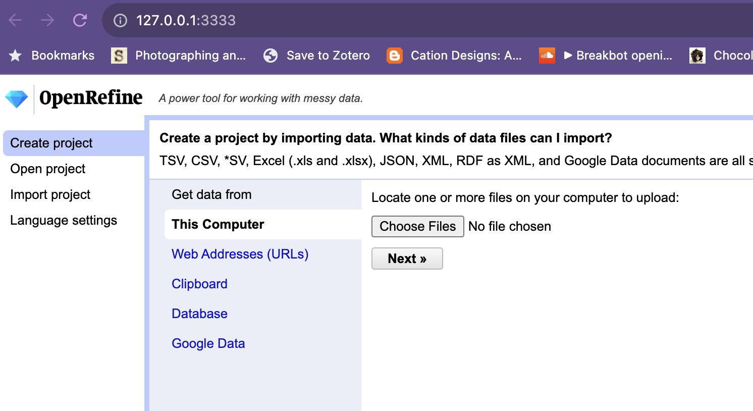
To get started, we can click on the Create Project button and then select the dh_conferences_works.csv file that we downloaded earlier.

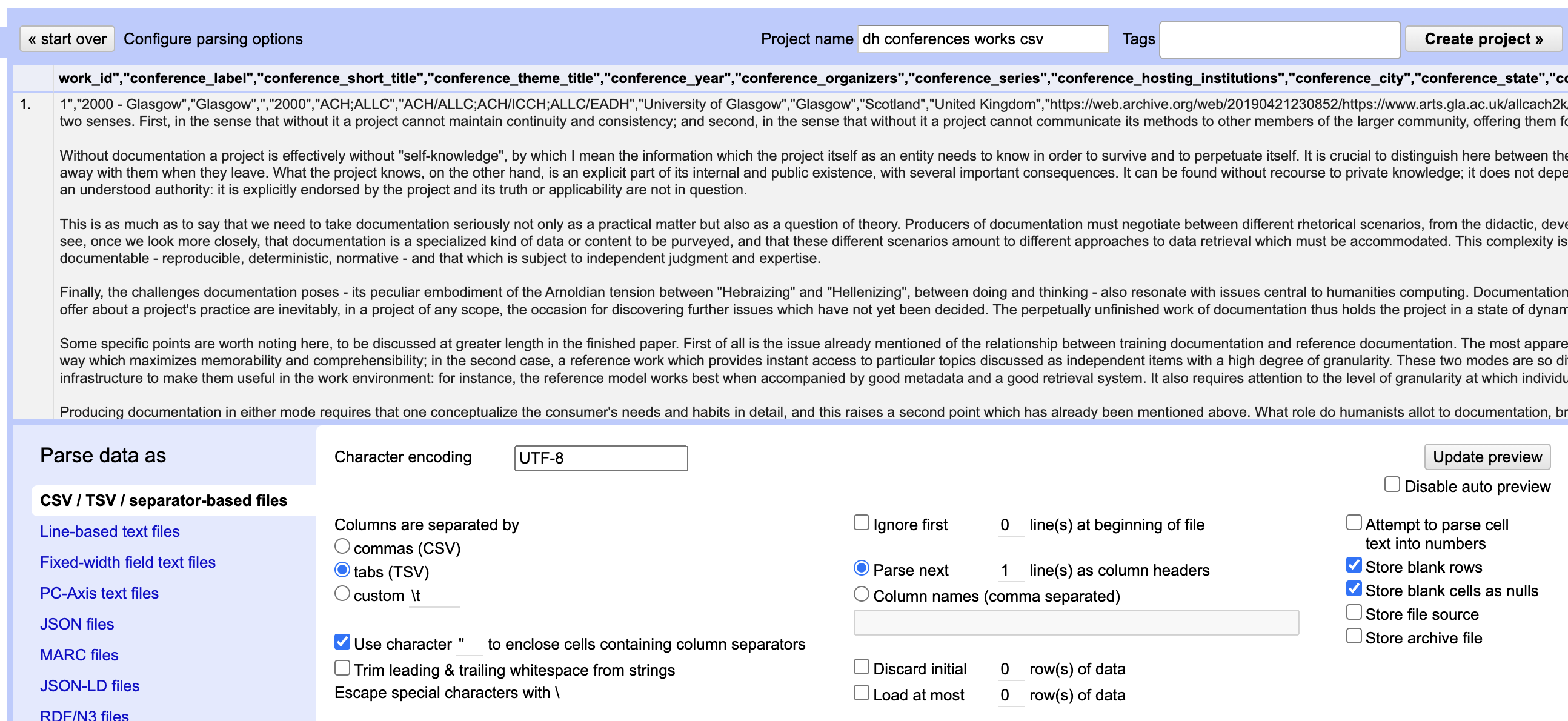
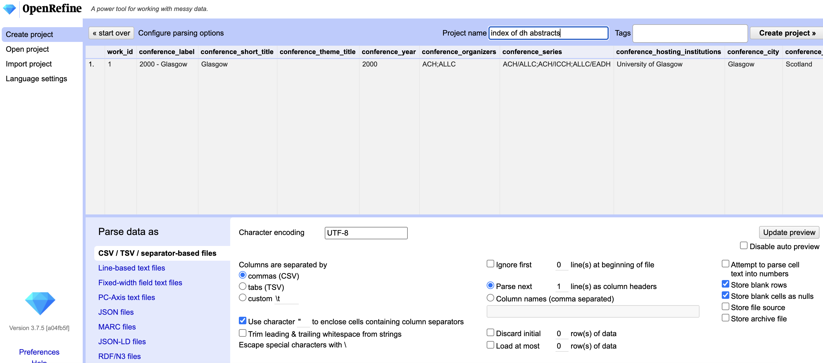
You’ll notice that it is currently struggling to parse our data into individual cells (it is all clumped together in the preview). To fix this we need to tell OpenRefine that our file is a csv (that is our data is separated by commas, not tabs – like a tsv file) and then we can also name our project in the top right hand side.

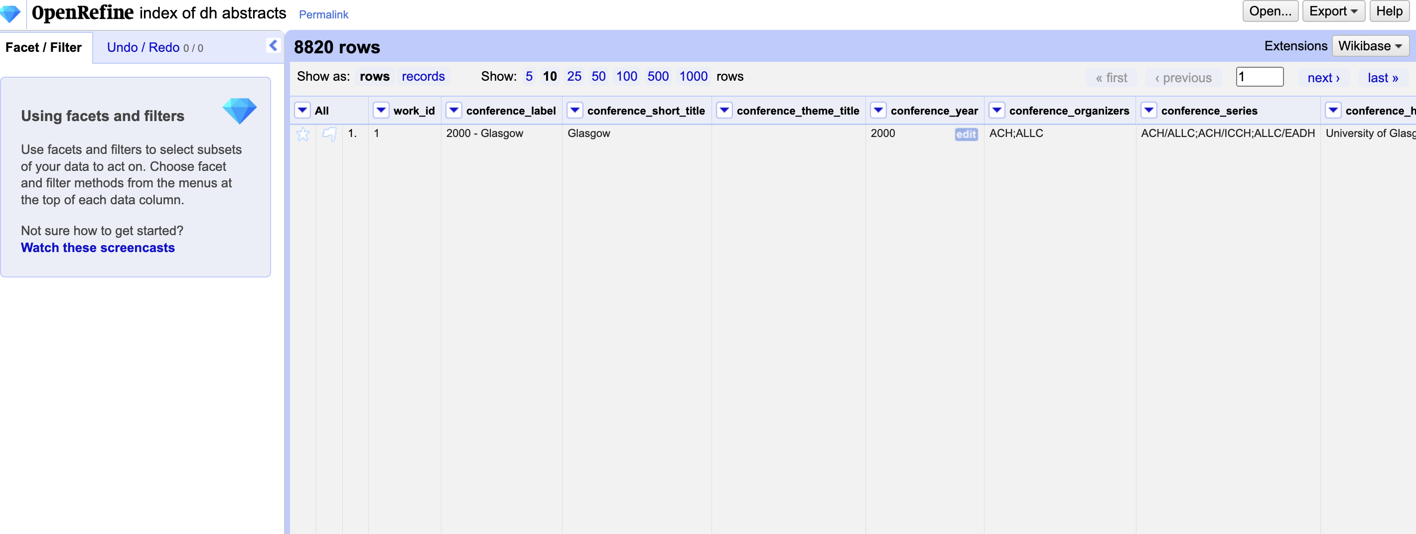
Now we should see our full dataset of 8820 rows and we can start exploring it through the OpenRefine interface.

To learn more about what OpenRefine can do, we should first explore the documentation: https://openrefine.org/docs/manual/exploring

Facets and Transforms

While the Overview section provides some helpful information about data types, the most important section is on Facets. One of the most powerful features of OpenRefine is the ability to use facets to explore your data. Facets are a way of filtering your data based on a specific column or value. For example, we can use the facet functionality to see how many unique values there are in the conference_label column, one of the required columns according to the documentation.

To try this out, we can click on the conference_label column and then click on the Facet button in the top right hand corner. This will open up a new menu on the left hand side that will allow us to explore the data. Then we can click on the Text Facet button to see the unique values in this column, through a popup box on the left hand side. We can also click on the Count button to sort the data and see the top values in the dataset.

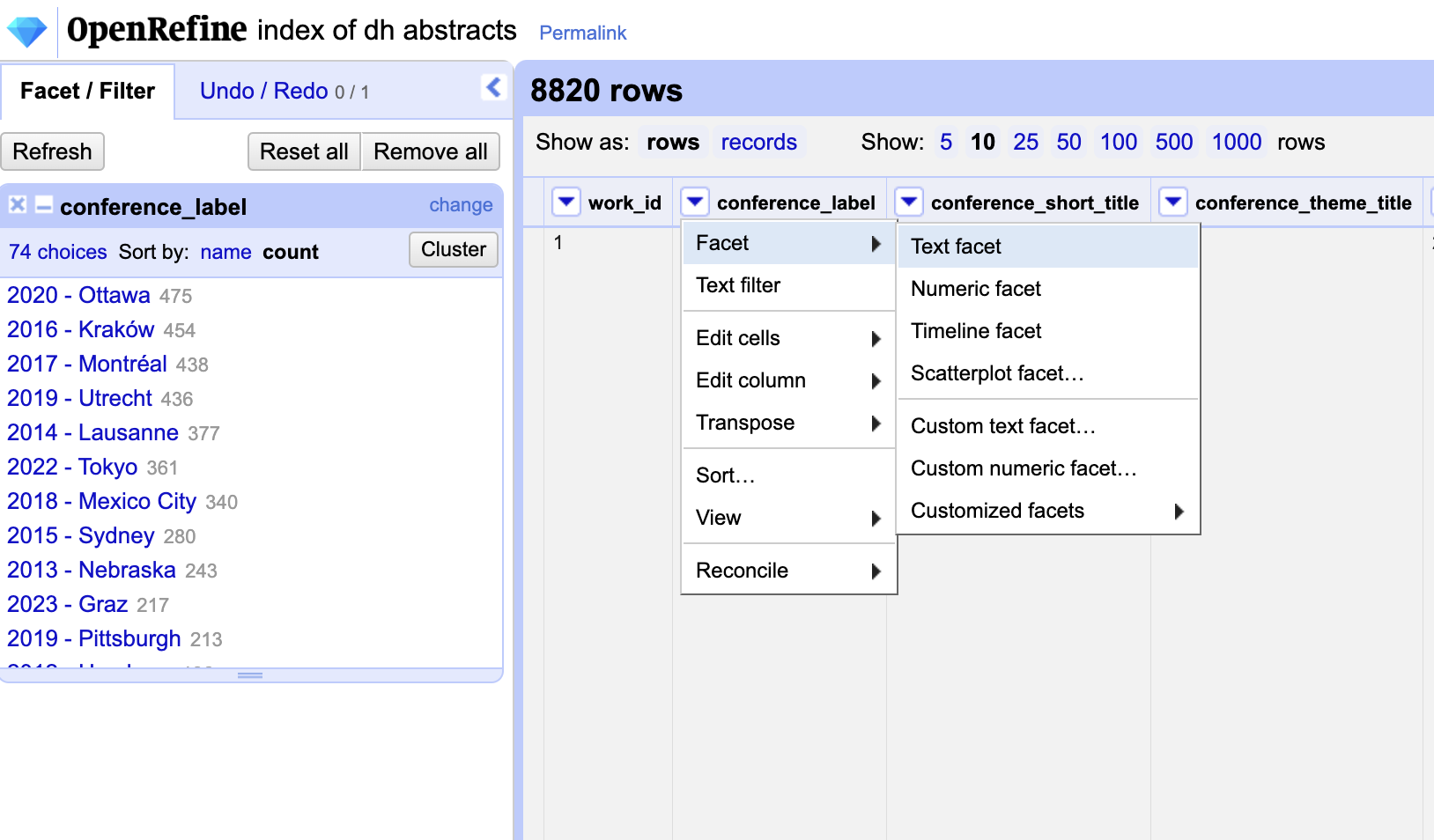
From this feature, we learn that we have the top amount of rows from the 2020 DH Conference in Ottawa. We can also click on the 2020 DH Conference in Ottawa value to see all the rows that contain this value.

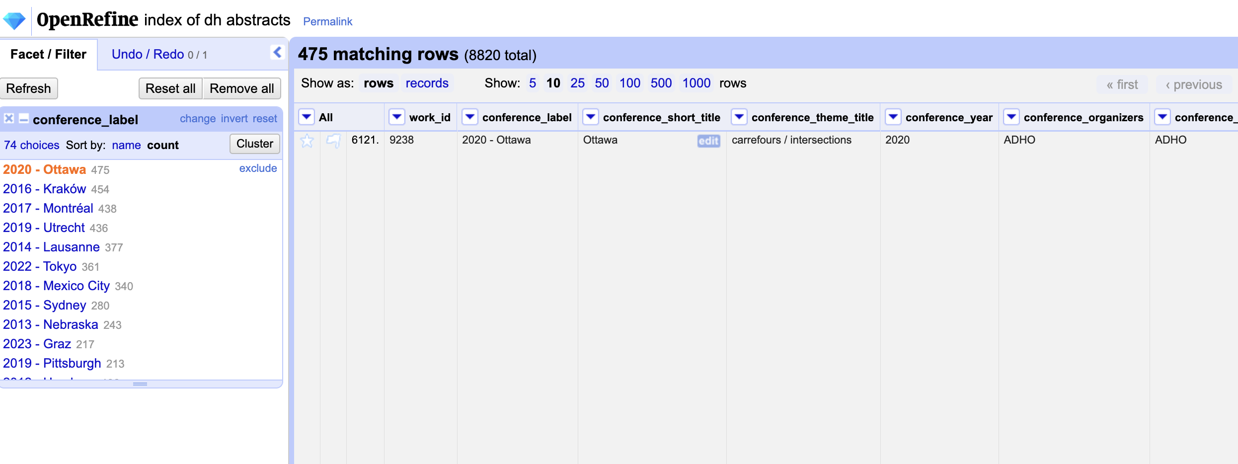
We can press the x button to remove this facet and return to our full dataset. We can also use the Text Facet functionality to explore other columns like conference_year or conference_city.

In addition to the Text Facet functionality, we can also use the Numeric Facet functionality to explore the conference_year column. This will allow us to see the range of values in this column and also to sort the data by the number of rows that contain each value.

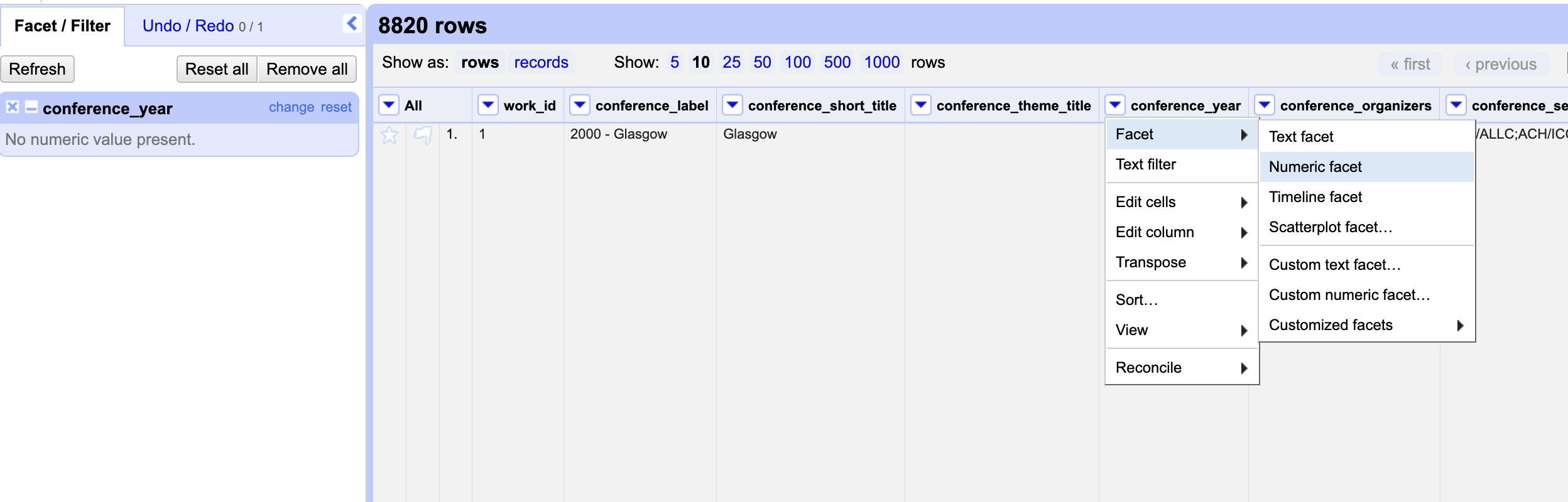
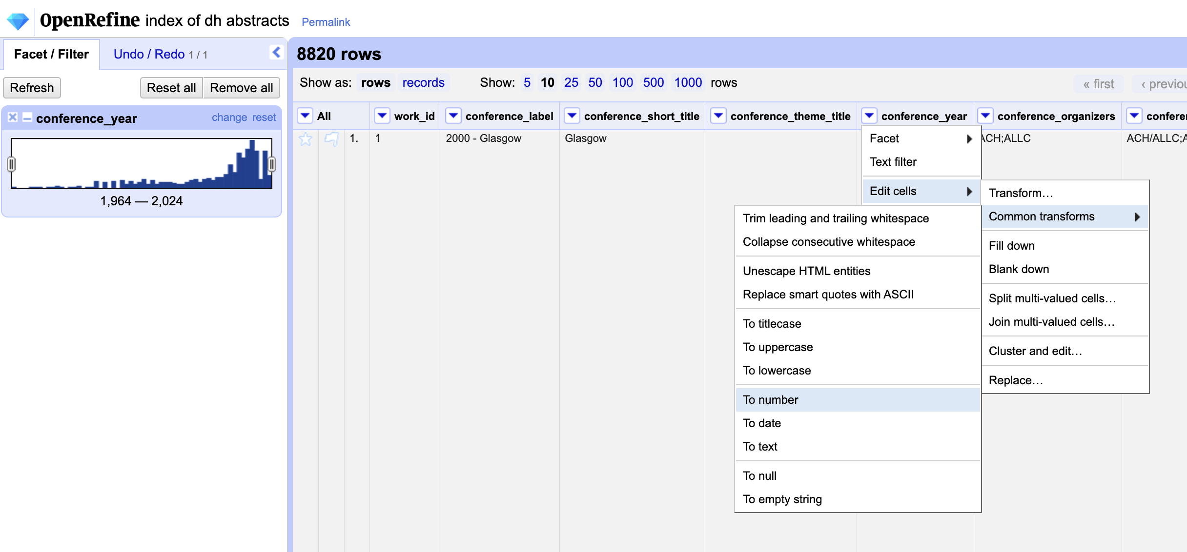
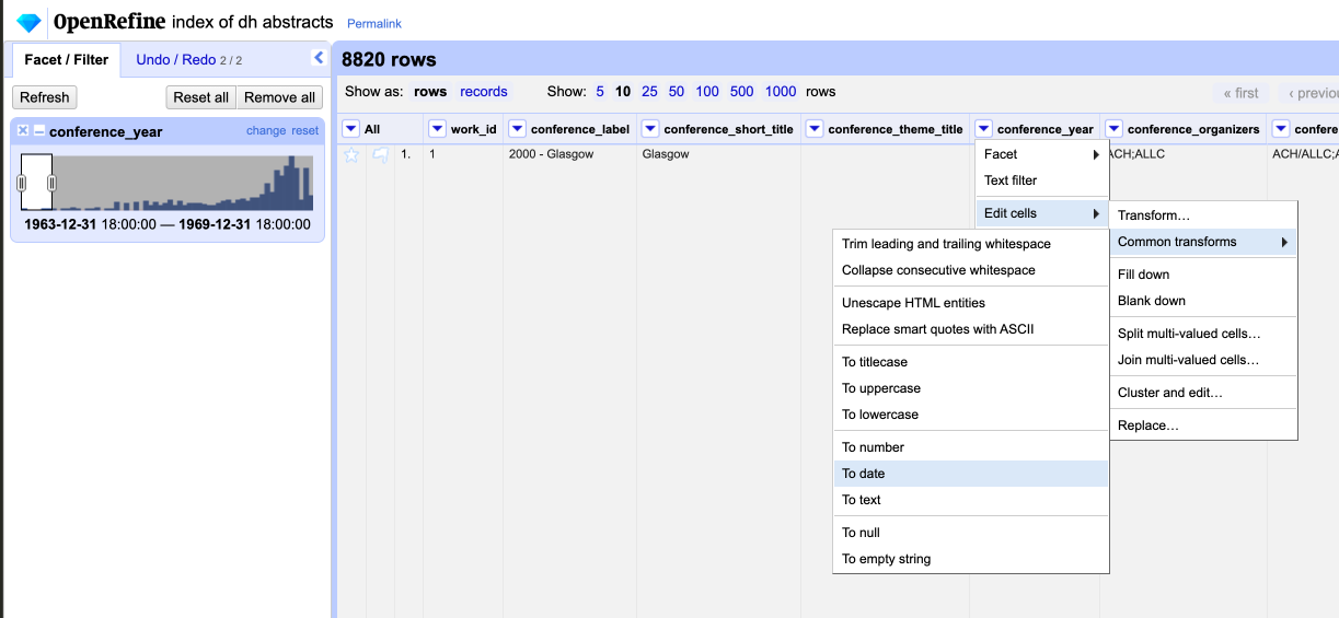
However, you’ll notice that when we try to use this filter we get an error message. This is because OpenRefine is trying to treat the conference_year column as a text column, not a numeric column. To fix this we need to use the Edit Cells functionality to change the data type of this column. We can read how to do this in the docs: https://openrefine.org/docs/manual/cellediting.

Essentially we want to turn our string into a number, so through selecting edit cells, and then common transforms, we can find the To number option. This will allow us to convert our string into a number.

Now we should see that we have a numeric facet that allows us to explore the conference_year column. But notice that it is treating years as numbers rather than a date. We can also try instead using the Timeline Facet functionality to explore this column.

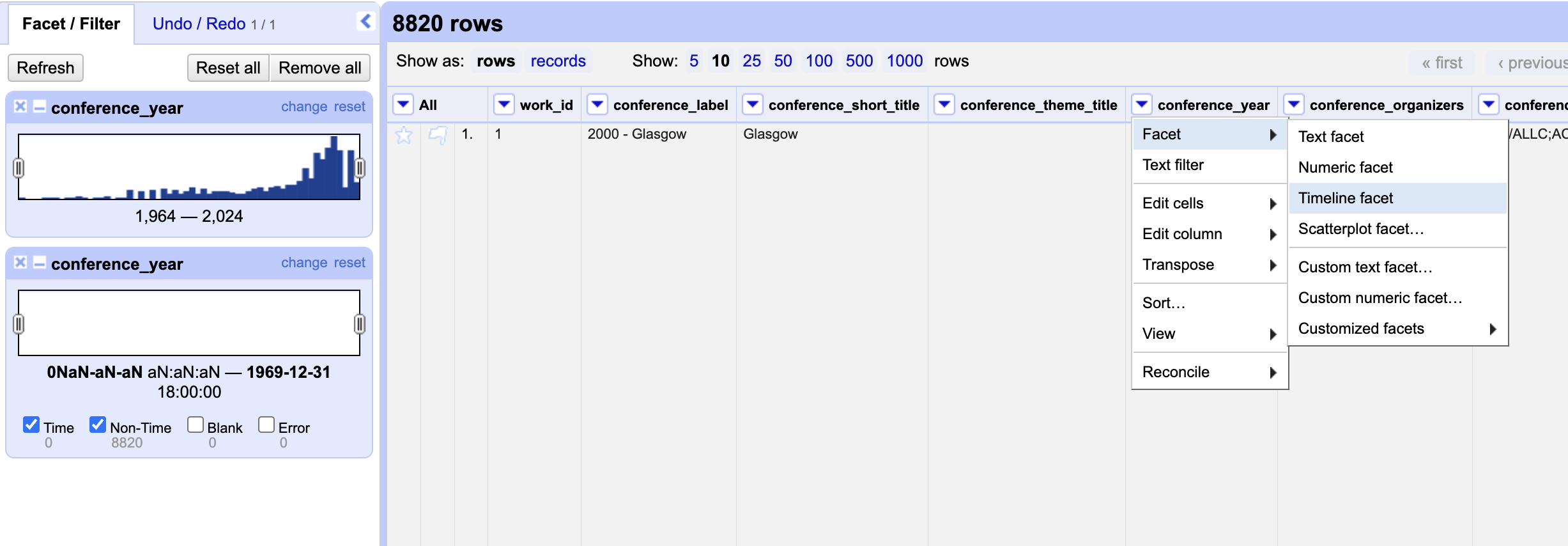
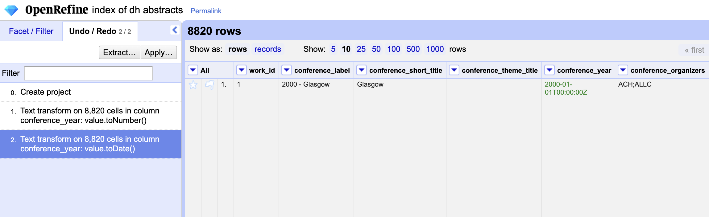
But now we are again getting an empty timeline. This is because OpenRefine is treating our column as a number, not a date. To fix this we can use the Edit Column functionality to change the data type of this column. First we should remove the Numeric Facet and then once again transform our data.

Now our data is correctly formatted and facetted, and we can even use this interface to filter our data by year.

We can also undo our transformations if you click on the Undo / Redo button in the top right hand corner. This will allow you to see all your changes, and reverse any changes you have made to your data.

Filtering and Deriving Data with OpenRefine

So far we have started to explore the functionality of this platform, but we also want to ultimately merge this data with our existing dataset. One of the issues is that currently OpenRefine does not allow you to merge datasets, so we will need to export this data and then merge it with our existing dataset in Google Sheets. You can read more about this missing functionality that used to exist in this tool and is proposed to be added in the GitHub repository for OpenRefine https://github.com/OpenRefine/OpenRefine/issues/5393.

But prior to exporting we need to think about how we plan to merge our datasets. Similar to our last example, we need to consider what would be a column that shares similar values.

In our dh tools dataset we have two potential candidates: either the link_dh_abstract or abstract_title. We can try using the link_dh_abstract column first, but we will need to clean it up a bit first.

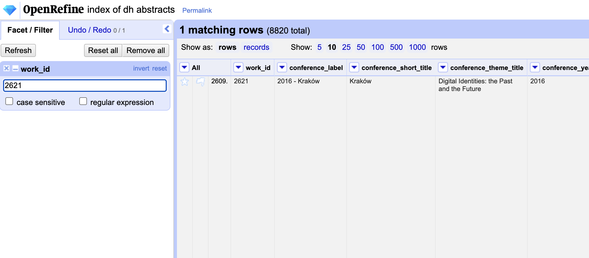
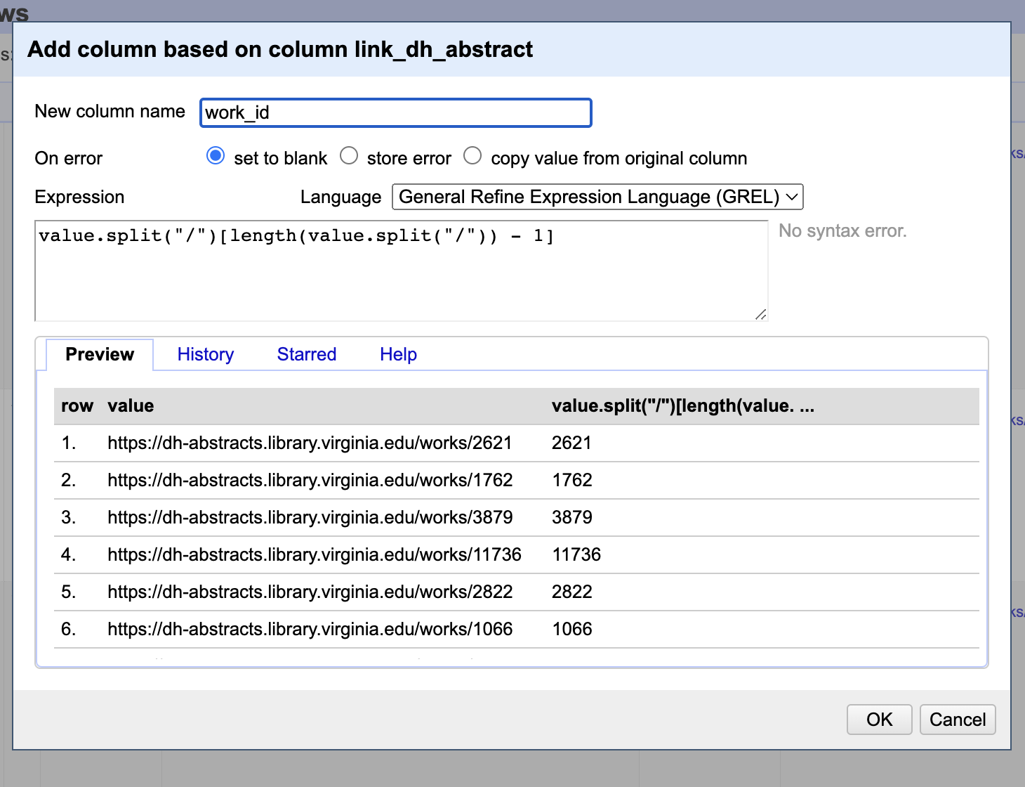
If you notice the link_dh_abstract column contains urls that have the following structure https://dh-abstracts.library.virginia.edu/works/2621 where the number at the end is the unique identifier for each abstract. We can use this to create a new column that only contains the number at the end of the url.

Let’s test this out first by using the filter functionality in our index dataset to only show the rows that contain the id above.

Now that we know this logic works, we can create a new column in our DH Tools dataset to contain only the work_id derived from the link_dh_abstract column. We could do this either in Google Sheets or OpenRefine if we loaded our data into OpenRefine.

OpenRefine Derive Column

If using OpenRefine, we first need to export our data from Google Sheets and upload it as a new project in OpenRefine as a project called DH Tools. Then we can use ChatGPT to help us with the following prompt:

I have an OpenRefine Project called DH Tools that has a column called linked_dh_abstract and that contains values formatted like the follow https://dh-abstracts.library.virginia.edu/works/2621. I want to create a new column called work_id that only contains the number at the end of the url. How can I do this?

We get the following instructions from ChatGPT:

To extract the number at the end of the URL in OpenRefine, you can use a combination of OpenRefine’s GREL (General Refine Expression Language) functions. The task essentially involves parsing the string to get the characters after the last forward slash (/).

Here’s how you can do this:

1. Open Your Project: Open your “DH Tools” project in OpenRefine.

2. Create a New Column:
   • Click on the dropdown arrow next to the linked_dh_abstract column.
   • Choose Edit column > Add column based on this column...

3. Enter the GREL Expression: In the expression box, use the following GREL formula:

   value.split("/")[length(value.split("/")) - 1]
   

   Here’s a brief explanation of the expression:

   • value.split("/"): This splits the URL at each forward slash, creating an array of elements.
   • length(value.split("/")) - 1: This finds the index of the last element in the array.
   • The whole expression thus extracts the last element of the array, which is the number you want.

4. Name the New Column: Enter the name work_id for the new column.

5. Apply Changes: Click on the OK button to apply the changes.

The new column, work_id, should now appear in your dataset, containing only the number at the end of each URL from the linked_dh_abstract column.

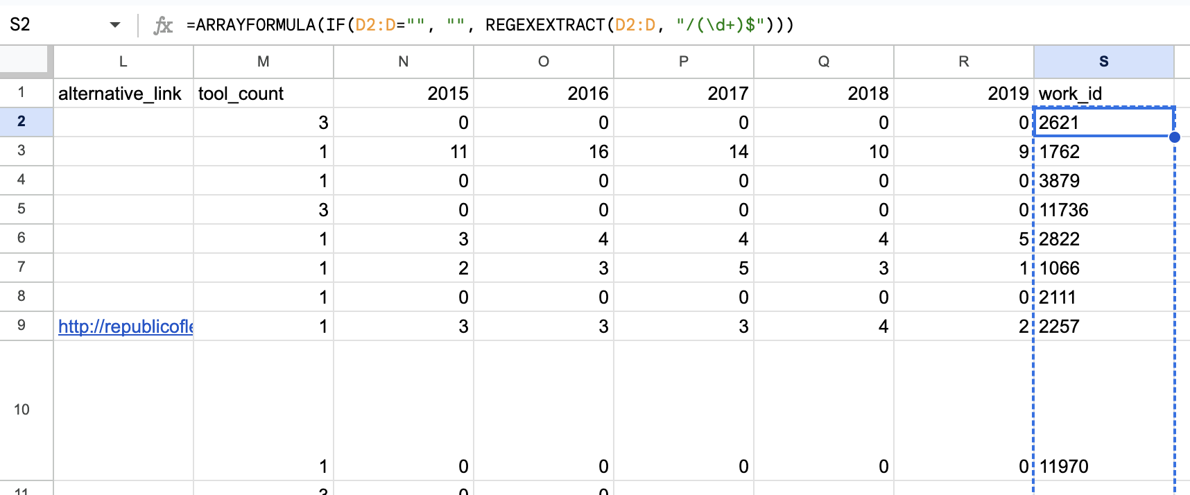
Google Sheets Derive Column

If using Google Sheets, we can use ChatGPT to help us with the following prompt:

I have a Google Sheets dataset called All DH Tools Revised with a column called link_dh_abstract that contains values formatted like the follow https://dh-abstracts.library.virginia.edu/works/2621. I want to create a new column called work_id that only contains the number at the end of the url and that column will be from the range S1:S18, whereas linked_dh_abstract has the range of D1:D18. How can I do this?

We get the following instructions from ChatGPT:

To extract the number at the end of the URL in Google Sheets, you can use a combination of Google Sheets’ built-in functions. The task essentially involves parsing the string to get the characters after the last forward slash (/).

Here’s how you can do this:

1. Create a New Column:
   • Click on the + button at the bottom-left of the Google Sheets interface.
   • Name the new column work_id.

2. Enter the Formula: In cell S2, enter the following formula:

   =ARRAYFORMULA(IF(D2:D="", "", REGEXEXTRACT(D2:D, "/(\d+)$")))
   

   Here’s a brief explanation of the formula:

   • REGEXEXTRACT(D2:D, "/(\d+)$"): This formula extracts sequences of numbers (represented by \d+) that appear at the end of a string (represented by $). The number sequence should follow a forward slash /, as seen in your URL format.
   • ARRAYFORMULA: This wraps around the REGEXEXTRACT function to apply the regex extraction to the entire column range.
   • IF(D2:D="", "", ...): This checks if a cell in column D is empty and, if so, ensures the corresponding cell in column S remains empty. Otherwise, it applies the regex extraction.

Regardless of how you generate this new column, once we have work_id in our dataset, we can use this column to filter our data with the Index of DH Conferences dataset with the help of ChatGPT and OpenRefine.

We want to use the Text Filter in OpenRefine with our Index of DH Abstracts Project to filter our data by the work_id column. We have already used this filter to try and find the work_id from the linked_dh_abstrct url. So we can try adding more work_ids to our filter by clicking on the work_id column and then selecting Text filter. Finally we can start adding our ids by simply copying them from Google Sheets.

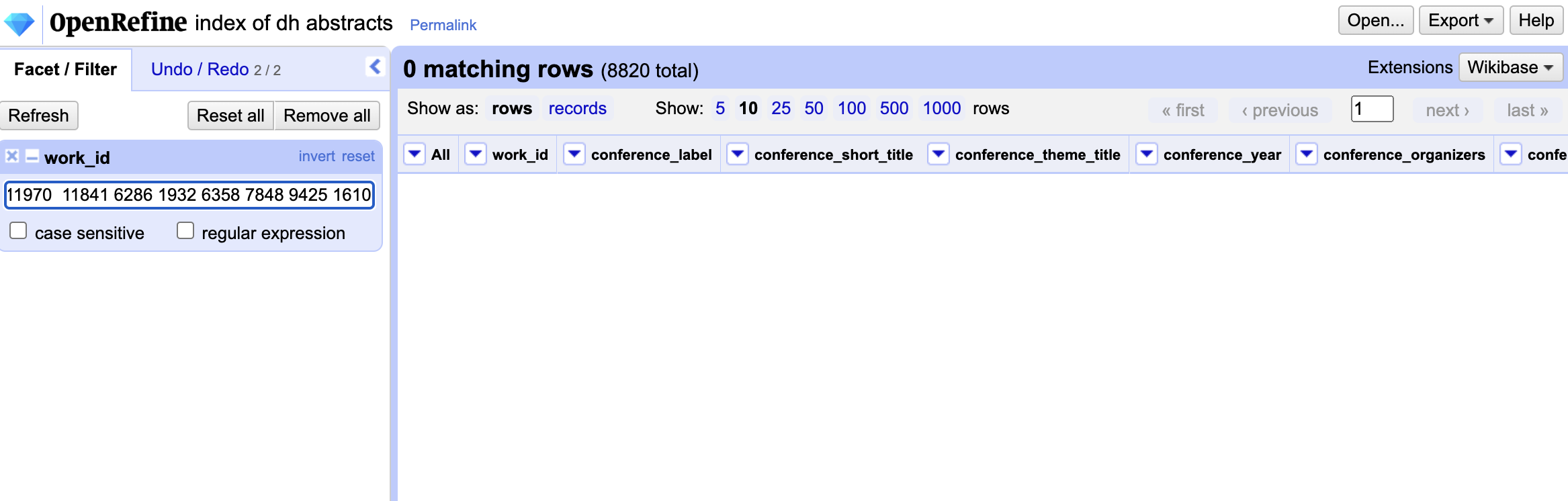
But you’ll notice that if we just enter multiple ids, then we end up with no rows or results. That’s because OpenRefine is trying to find rows that contain all of the ids we entered. Instead we want to find rows that contain any of the ids we entered. We can ask ChatGPT for help with this by using the following prompt:

I have an OpenRefine Project called Index of DH Abstracts that has a column called work_id that contains values like 2621. I want to filter this dataset by multiple values in the work_id column. How can I do this?

With the following answer:

In OpenRefine, filtering by multiple values in a column can be achieved using a text filter with a regular expression. Here’s how you can filter the work_id column by multiple values:

1. Open Your Project:

   Launch OpenRefine and open your project named “Index of DH Abstracts.”

2. Access Text Filter:

   Click on the downward arrow next to the work_id column header. From the drop-down menu, select Text filter.

3. Enter the Regular Expression:

   In the text filter box that appears, enter a regular expression that matches the values you want to filter by. For example, if you want to filter by the work_id values 2621, 1762, and 3879, you would enter:

   ^(2621|1762|3879)$
   

   Explanation:

   • ^: Matches the beginning of the string.
   • $: Matches the end of the string.
   • |: Acts as an OR operator in regex.
   • (2621|1762|3879): Matches any of the provided values.

4. Apply the Filter:

   Once you’ve entered the regex, the rows that match the provided work_id values will be displayed, and the rest will be filtered out.

5. View or Export the Filtered Data:

   With the filter applied, you can view, edit, or export the data as needed.

6. Remove the Filter:

   If you want to go back to viewing all rows, simply click on the “x” or “clear” button in the text filter box to remove the filter.

This method lets you filter by multiple values in a column efficiently. If you have more values to filter by, simply add them to the regex using the | operator. This special symbol is called a pipe or | and tells OpenRefine to filter any rows that contain any of these values. We can read more about this in the docs: https://openrefine.org/docs/manual/facets.html#text-filter.

We can even use ChatGPT to take our list of work_ids:

2621
1762
3879
11736
2822
1066
2111
2257
11970

11841
6286
1932
6358
7848
9425
1610

And turn it into a regular expression that we can use in OpenRefine:

^(2621|1762|3879|11736|2822|1066|2111|2257|11970|11841|6286|1932|6358|7848|9425|1610)$

Now we can use this in our Text Filter:

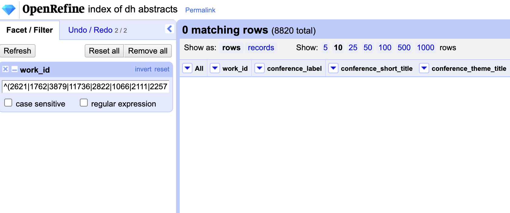
Initially we will still have empty values, but if we click the regular expression button, then we should see our filtered data.

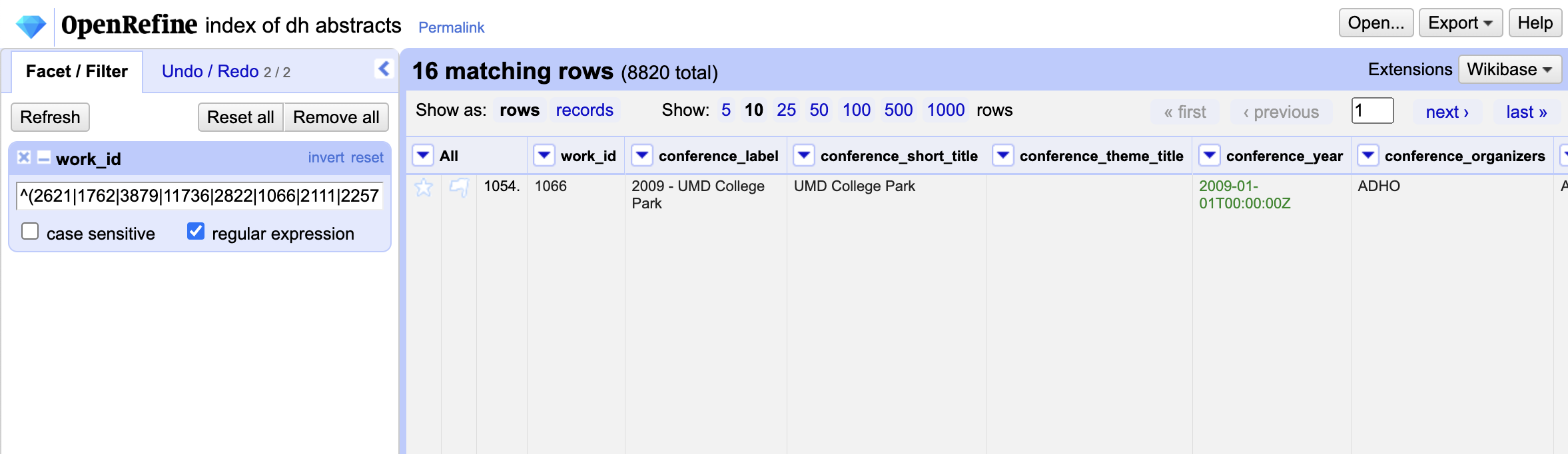
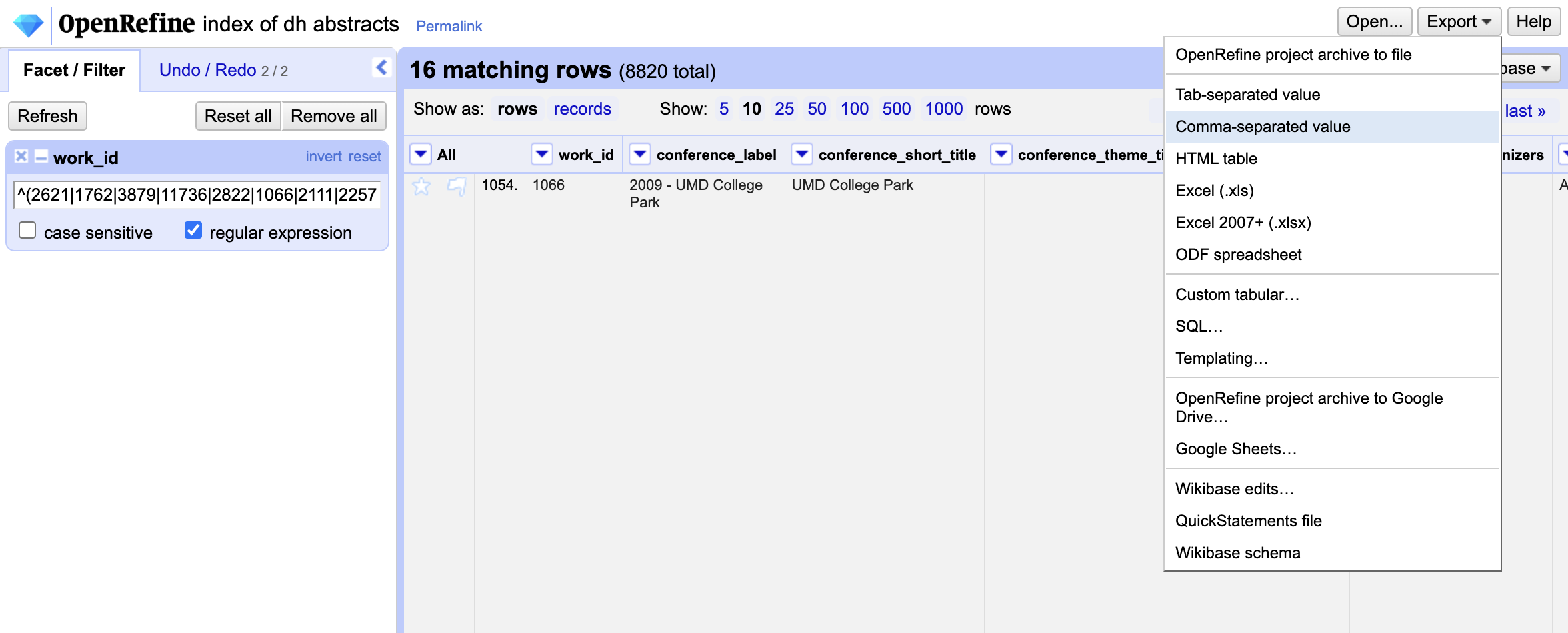
Now we have our filtered dataset (we only have 16 rows, since our dataset had 18 rows with one missing work_id and one row of headers), and now we can export our filtered dataset to finally merge it with our dh tools dataset using the same VLOOKUP process.

Data Cleaning and Merging Assignment

Part 1: Completing Data Merging (Optional Assignment)

This assignment is somewhat advanced so it is technically optional though I think you are all capable of undertaking this work. But we will also go through it at the start of our workshop in class just to make sure everyone is understanding how we merge and transform data.

If you decide to try it out for this assignment, you will complete the final merging process of dh tools with the Index of DH Abstracts dataset. I have provided the example Google Sheets dataset that has all the steps up to now, as well as the filtered dataset from OpenRefine. You can find these datasets here:

• DH Tools dataset
• Index of DH Abstracts

Now you need to complete the following steps:

1. Create a copy of the example Google Sheets dataset and rename it to dh tools merged.
2. Import the subset of index of dh abstracts dataset into your Google Sheets
3. Now start trying to merge the datasets with the help of ChatGPT and the examples above. You should be sure to include the following information in your prompt:
   • The name of your respective sheets
   • The name of the columns you want to merge
   • The range of the columns you want to merge
   • The name of the new sheet you want to create
   • The name of the shared column that you want to use to merge the datasets

Part 2: Experimenting with Data Cleaning

If you aren’t feeling comfortable doing VLOOKUP merges yet that’s completely ok! Instead, in this assignment you will start experimenting with OpenRefine.

1. Download the simple csv dataset from here https://dh-abstracts.library.virginia.edu/downloads and that should download a zip file that when opened contains a csv file called dh_conferences_works.csv.
2. Install OpenRefine https://openrefine.org/download and then create a new project with the dh_conferences_works.csv file.
3. Start exploring the data using the Facet functionality in OpenRefine. You can read more about this functionality here: https://openrefine.org/docs/manual/exploring
4. Transform the data so that conference year is an actual date.
5. Try using the Text Filter functionality to filter the data by one or two DH Tools that you are interested in. You can read more about this functionality here: https://openrefine.org/docs/manual/facets.html#text-filter. You will need to decide which column to filter on and should aim to have a dataset that is no larger than 200 rows but no smaller than 5 rows.
6. Export your filtered data as a CSV and share it with the class, either through uploading it directly to GitHub or sharing a link to a Google Sheets version. All links should be shared in the GitHub discussion https://github.com/ZoeLeBlanc/is578-intro-dh/discussions/4.

Additional Resources

• “OpenRefine for Natural History Collection Data.” https://data-lessons.github.io/OpenRefine-nhcdata-lesson/.
• Miriam Posner’s Get Started with OpenRefine https://github.com/miriamposner/get-started-with-openrefine/blob/master/get-started-with-openrefine.md (also available as a video https://share.descript.com/view/5Hx7a2XNWbW?t=1.470981&autoplay=1)